CHAPTER 7
Master Data Modeling

At this point in our MDM architecture discussion, we are ready to take a closer look at a particularly important and foundational concern of any data management framework—the discipline of data modeling and specific issues related to data modeling in MDM environments.

Importance of Data Modeling

In the corporate world, enterprise data resides mostly in relational databases. Similarly to the cities, towns, villages, housing developments, and individual buildings that require architects to create the structures and then control structural changes, the organization of data requires sound architectural standards and principles. Data modeling is the key part of data architecture that defines the structures in which the enterprise data resides and evolves. Enterprise data modeling is considered a powerful technique to define, create, and maintain data structures and enable data integrity; gather business requirements; and communicate and socialize the scope of enterprise data; its organization, levels of aggregation, and constraints.

Furthermore, a robust and scalable data architecture enables meaningful and timely change. Historically, every era has witnessed an accelerated rate of change and scope from many perspectives such as business, technology, regulatory, social, and political. To flourish or even simply survive in this environment requires real business agility to respond to market threats and opportunities as well as regulatory challenges. Strategic and tactical business strategies, business operations, and supporting technologies must all be malleable and aligned.

Over the past four decades, since Edgar F. Codd introduced the notion of a relational database and its normalization principles,^1–3 data modeling has evolved into a discipline that defines a common data modeling “language” widely accepted by various enterprise users: data modelers, business analysts, database administrators, application and database developers, data governors, and data stewards. Data modeling is used in a variety of contexts and scenarios, ranging from conceptual and canonical models that determine the entities and relationships in a system-agnostic way, to logical and physical data models that represent specific systems and applications.

For a data modeler, a data model provides valuable business and architectural insight into the scope of the enterprise data, data integrity rules, information on how the data modeling universe will be able to support business processes and determine what data can be retrieved, and the paths to join pieces of information to bring them together. For business and systems analysts, a data model can play an important role in gathering and documenting business requirements.

Data modeling tools supporting modern physical data models allow database administrators and database developers to model and maintain a variety of objects (tables, indexes, attributes of various data types, views, triggers, stored procedures, functions, constraints, and other more complex objects) for an assortment of database vendors and products.

In order to support a variety of needs and views at different levels of abstraction and granularity, the data modeling discipline introduced a number of modeling styles that differ by the goal for which each of the styles is optimized. In this chapter we briefly discuss the styles that dominate the current data modeling market. We concentrate on the strengths of these data modeling styles and some of their weaknesses, especially as these weaknesses apply to Master Data Management, which is the focus of this book.

We analyze master data modeling–specific needs to understand which data modeling methodologies, techniques, and patterns developed over the decades are best fit to model the master data, and how. Then, based on this analysis, we focus on the modeling styles in the context of their relevance and optimization for master data. This will help us arrive at conclusions as to what data modeling styles can be used for different master data solution scenarios. We discuss a number of practical and important master data aspects around the dependencies between MDM data modeling styles and the goals they have to support, including such important considerations as change control issues, data model readability, required history support, and support for entity resolution and relationship resolution, and contrast this with the needs of applications that consume MDM services, on-going support for master data model synchronization, and so on.

Predominant Data Modeling Styles

The third normal form (3NF) modeling introduced by Edgar F. Codd has been the most widely adopted standard for several decades. The 3NF normalized models are optimized to ensure minimal data redundancy. For instance, if a doctor’s office or hospital captures and re-enters the patient’s name, address, date of birth, and other static or infrequently changing pieces of information for every patient visit, along with visit-specific information, the patients’ data will be redundant. Not only will such redundancy require extra data storage; what is more important, data redundancy may cause data inconsistencies and complicate data maintenance. Indeed, if a data element value is incorrect, in order to fix the issue the data must be corrected in multiple places where the data element is stored. Similarly, if a company’s order processing system requires or allows the information about its frequent customers to be re-entered every time a customer places an order or opens a new account, this situation will lead to data redundancy.

The burden and subsequent costs to an organization are often significant. Change is stifled. Redundancy masks the fundamental problem of accessing an entire data domain in terms of its original purpose and also utilizing it for new business purposes.

Data normalization techniques and 3NF normalization techniques, specifically, tackle the problem by breaking large data into relatively small normalized tables where the data attributes depend on the primary key and only the primary key. For example, an Order table that contains both customer- and order-level data in its denormalized form may be split into two tables as a result of normalization. These are the Customer table and the Order table, with the customer-specific attributes residing in the Customer table while the order-specific attributes remain in the Order table. The Order table would have a reference key (foreign key) that points to a uniquely identified customer in the customer table.

Because 3NF modeling minimizes or eliminates data redundancy, the 3NF modeling style is considered a good choice for transactional systems, where the primary goal is to input and update the data in the database and maintain the data consistency. When the data is stored without redundancy, data consistency issues are addressed naturally. Expressed differently, 3NF is the preferred and predominant modeling style for On-Line Transaction Processing (OLTP).

If the goal of data modeling is to optimize the data model for reporting and analytics, a normalized model may not be the best choice. With the data modeled in the 3NF format, bringing data from different tables together for a report may require many tables to be queried in a joint fashion (in RDBMS, this operation is called a “join,” and it can be a very expensive operation in terms of computing resources and the performance impact). In addition to the potential performance problems, joins represent challenges for the database developer responsible for making the tables to join with each other correctly and efficiently, using the least amount of resources and creating a minimal an amount of intermediate, temporary tables as possible.

As the cost of storage dropped significantly over the last several decades, enterprises started gathering increasingly more information about their businesses, customers, products, and other data domains, both broader in scope and deeper in the detail levels of granularity. This has resulted in the material increase in the number of data records, elements, and attributes that need to be stored and processed. From the data modeling perspective, this trend that started in 1990s led to a tremendous increase in the complexity of enterprise data models, often having to manage thousands of entities and relationships in a single model.

In an extreme case, one simple report metric, such as total sales, can span numerous tables from multiple internal and external sources in multiple geographic and functional domains. Moreover, each of these data sources can have different technical architectures and different business definitions.

Figure 7-1 illustrates a typical representation of a 3NF data model with the number of entities around 50.

Even with 50 entities, it is not easy to navigate through such a model and correctly join the tables to retrieve the results of a complex reporting query. When the number of tables grows to reach hundreds and even thousands of tables or entities, the complexity of the model defeats the purpose of the data model stated at the beginning of this chapter as a common “language” that can be used by many data modeling stakeholders across the enterprise.

Robert Hillard⁴ proposed measuring the complexity of the data model by looking at it as a graph within the Small World theory. The Small World theory had been earlier applied to networking in biology, sociology, telephony, and other types of networks. The theory evaluates the complexity of the network in terms of the number of steps required to assemble information distributed across the network. The Small World approach uses the graph theory terms vertex (node) and edge (connection between nodes). These two terms can be easily interpreted in terms of the more traditional data modeling concepts of entity and relationship, respectively. This approach introduces the following terms:

• Vertex (node) = entity

• Edge (connection between nodes] = relationship

• Order = number of entities/vertices

Enterprise data modeling is considered a powerful technique to define, create, and maintain data structures and data integrity, and communicate and socialize the scope of the enterprise data, its organization, and its levels of aggregation and constraints.

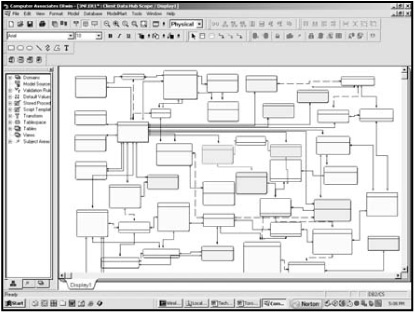
FIGURE 7-1 An illustrative example of a normalized data model

• Enterprise data models, when 3NF normalized, include many hundreds and oftentimes thousands of entities connected in many different ways.

• Simple business questions become very difficult with the 3NF enterprise model.

• There are no clearly defined processes and procedures for how the data model is going to be used and maintained.

• Expensive industry data models oftentimes end up unused.

• Size = number of relationships/edges

• Geodesic distance = minimum number of relationships/edges to be traversed

• Average degree = average number of edges (connections) per node

• Average distance = averaging the geodesic distance of all entity pairs

• Maximum distance = maximum number of edges/relationships needed to traverse between the two most remote entities in the model

Figure 7-2 illustrates the concept of the Small World theory and its metrics.

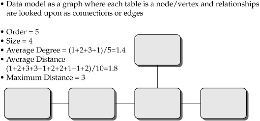
FIGURE 7-2 The Small World theory metrics

From more traditional data modeling and database development perspectives, these measures evaluate a potential complexity of the joins that may be required to bring the data together and to read the model intelligently. The theory suggests that if the average geodesic distance is less than 4, the graph (in this case, the data model) is relatively easy to read and navigate. A graph with an average distance approaching 10 makes it extremely challenging to navigate the model, even for individuals who do it on a daily basis as a full-time job. Hence, in order for multiple stakeholder groups to use the data model as a common language, the average geodesic distance should not exceed 4. The data model with an average geodesic distance between 4 and 10 can be used only by trained and tenured database developers and administrators. As the average geodesic distance approaches 10 and exceeds it, the data model as a readable network environment becomes inefficient.

NOTE 3NF is not the only normalization modeling schema, just the most popular. Other, next-level normalization forms exist, with 4NF addressing normalization that considers multivalued dependencies⁵ and 5NF designed to reduce redundancy related to multivalued facts.⁶ These are very advanced normalization topics. They are beyond the scope of this book and have somewhat limited practical significance.

The aforementioned difficulties with the 3NF data modeling design drove the need to develop alternative data modeling techniques optimized for data retrieval, reporting, and decision making. The star schema modeling approach was championed by Ralph Kimball in his first data warehousing book⁷ and the books and numerous articles that followed.

FIGURE 7-3 Illustration of the star schema design

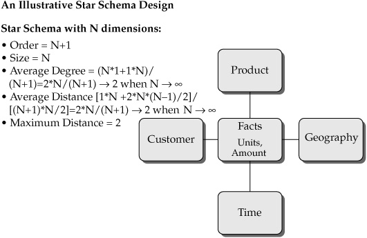
The star schema modeling is optimized for data retrieval and therefore is much better suited to support business intelligence, analytics, data warehousing, and ultimately decision making. Consequently, the star schema modeling design is often considered as an integral part of On-Line Analytical Processing (OLAP). We have briefly mentioned the concept of a star schema data model as it relates to data warehousing in Chapters 4 and 5. Figure 7-3 illustrates the typical star schema design.

This modeling design makes it much easier to read and retrieve data. The central table (fact table) usually holds numeric metrics—for example, sales revenue, sold units count, number of shipments, and so on. The tables around the center of the star are known as dimensional tables or dimensions (often representing reference data). The simple illustrative star schema in Figure 7-3 depicts Customer, Product, Geography, and Time dimensions. We will assume that the Time dimension is built with a granularity of calendar date, as is often done in data warehousing. Let’s assume that there are two metrics (facts) in the fact table. The first metric represents the number of units sold, and the second metric represents the amount spent by a customer on a specific product on a given date. This model is easy to read and is often interpreted using the “slice and dice” metaphor. It is intuitively clear that the structure is designed for reporting on unit counts and dollar amount spent by a given customer on a given product at a given geography or location on a given date. Note that even with millions of records in the data store, the star schema design can enable a sub-second execution time for the query:

select UnitCount from Facts, Customer, Product, Geography, Time, where
CustomerID = ‘Given CustomerID’,
ProductID = ‘Given ProductID’,
Geography = ‘Given GeographyID’,
TimeID = ‘GivenDateID’

Although this query joins five tables, as long as each join predicate can be evaluated using simple equality operator (=), the type of join where a large table in the middle of the star (fact table) is joined with its immediate neighbors (dimensions) turns out to be very efficient from the performance, readability, and ease-of-use perspectives. Consequently, all major database vendors have developed proprietary star-join query optimization techniques.

We can interpret readability and the ease of use of the star schema model in terms of the Small World theory.

In the preceding formulas, (1*N) stands for N distances equal to 1 between each of the N dimensions and the fact table. 2*N*(N–1)/2 comes from the contribution of N*(N–1)/2 distances between the dimensions, with each distance being equal to 2. (N+1)*N/2 is the total number of distances between N+1 nodes (one fact table and N dimensions).

A star schema design assumes that the fact table is much larger by data volume (and certainly by the number of records) than the dimensional tables. This drives the recommendation to keep the dimensions denormalized since data redundancy in dimensions does not significantly impact the overall database size because the volume of the fact table mainly determines the total volume of the database. Still, data modelers sometimes denormalize dimensions and connect them with related fact tables, which results in a design known as a “snowflake” schema.

Star and snowflake schemas are built on a common design principle: separation of facts and references about the facts into two connected types of structures—fact and dimension tables. To avoid confusion, we will refer to both of these model types using a common name: the dimensional model.

NOTE The assumption that the fact table is much larger in volume than dimensional tables doesn’t always hold true (for example, consider a customer reference data dimension that may contain millions of records and can grow significantly if there is a requirement for historical reference data). The trend has been to persist history, thus significantly increasing business value, but at the cost of increased complexity and performance burden.

It should be noted that the 3NF structures and the dimensional model structures are so different that it is not a recommended practice to gradually move your model between these two formats. Many modelers have tried it without success. Data modelers often maintain both model formats (that is, star schema and 3NF) to make sure that their transactional needs and reporting needs are adequately supported.

As we can see, data modeling design requirements depend upon the data model purpose. In addition to the widely known 3NF and dimensional model designs (that is, the star and snowflake schemas), some alternative data modeling techniques have been developed. For instance, data vault modeling for enterprise data warehousing has been gaining popularity over the last decade.⁸ It’s a hybrid approach that utilizes the concepts of 3NF and star/snowflake schema.

NOTE A number of data modeling design styles and levels of abstraction must be maintained by data modelers and architects to support a variety of data modeling purposes, roles, and stakeholder groups.

MDM Data Modeling Requirements

In the previous section we discussed the predominant data modeling patterns and reviewed the criteria of what scenarios these patterns are optimized for. Now we are in a position to focus on the key MDM data modeling requirements. These requirements will lead us to the master data modeling patterns and an understanding of what they can leverage from the normalization techniques, dimensional schema design, and other architecture patterns.

In the discussion that follows, we will assume that a master data model meets the following requirements:

• It must be optimized for entity resolution, relationship resolution, and fast searches of master entity records.

• It must be flexible to support multiple data domains with a variety of master entities and relationships.

• It should be able to support consuming applications such as data warehouses, data marts, operational data stores, and so on.

Let’s analyze these three requirements and use them as a guide to understand master data modeling principles and patterns.

One of the primary tenets of the previous chapters has been the idea of entity resolution and relationship resolution. In order to efficiently support entity resolution and relationship resolution, a master data model must be optimized to expose and manage master data entities, their keys and identifiers, and the dynamic relationships between the entities. As we already know, these entities include Party, Product, Location, Instrument, Organization, and other entities, where the record count is expected to be at least in the thousands and can climb to many millions and even billions. For some applications (such as Person of Interest in law enforcement, counterterrorism, and intelligence gathering), these entities can be more complex than the “classical” entity types listed above, as we discussed in Chapter 3.

It is important to understand that when we discuss MDM from the entity resolution perspective, the notion of an “MDM entity” is different from the notion of an “entity” in the 3NF world. In the 3NF world, it is assumed that there is a way to define a record uniquely and the modeler is not responsible for figuring out how this is going to be done. The 3NF model asserts the existence of the primary key for each entity while not specifying how this primary key is created or inferred. A traditional 3NF modeling process does not divide the attributes into those that will be used for matching, entity resolution, and relationship resolution and those that will not be used for these purposes. Technically speaking, two or more records can have totally identical nonkey attributes. This is perfectly “legal” from the 3NF perspective to have all identical non-key attributes while two or more records have different primary keys.

This is quite different in dimensional modeling. Ralph Kimball’s definitive book on the subject⁷ defines the key steps of how a star schema model is developed. The process begins with the identification of business flows that drive the selection of the facts and their granularity. Then the data modeler defines the dimensions, levels of aggregation, and so on.

Let’s follow this pattern by defining and discussing in detail the steps that need to be followed to develop the model optimized for entity resolution and relationship resolution:

1. Define entity domains. High-level definitions of these domains and the domain implementation sequence are typically aligned with and driven by business strategies. Party, Product, Location, Supplier, and Account are the most frequent candidates in the list of MDM data domains.

2. For each master data domain, define the entities that need to be resolved algorithmically due to their complexity. Let’s take a look at the entities and attributes of a Party model and discuss the differences in how these constructs are presented in the 3NF model and in the master data model optimized for entity resolution and relationship resolution. For example, for the Party domain we need to define what entities we will need to resolve algorithmically due to their volume and complexity and what entities we will extensively search on in MDM-enabled applications across the enterprise.

Unlike 3NF modeling, where all entities are equal and volume agnostic, master data modeling optimized for entity resolution concentrates on the entities that have high volumes of data and require advanced algorithms. We touched on these algorithm categories in Chapter 6 (probabilistic, machine learning, and so on). For instance, from the 3NF perspective, the entities Customer, Country, and Gender would normally be represented as three entities depicted as “boxes” in an Entity Relationship Diagram (ERD) with the primary keys CustomerID, CountryID, and GenderID. Unlike that, from the entity resolution perspective, the entity Customer (with thousands and oftentimes millions of records) is typically the “first-class citizen” that requires an entity resolution algorithm, whereas entities such as Country and Gender do not qualify for this “first-class citizen” entity category.

Many enterprises serve both individual and commercial or institutional customers. This makes “Individual” and “Organization” the most likely candidates for the “first-class citizen” entities in the Party domain. An identification of the “first-class citizen” entities must take into account business definitions of the terms “Customer,” “Product,” and so on. An enterprise division or line of business that services retail customers (individuals), in addition to having individual customers in the MDM Data Hub, may also want to see “Household” as a separate entity to support marketing needs. For many organizations and business functions, the notion of a Household is a preferred definition of a Customer. The division that serves commercial customers may have multiple definitions of the entities comprising the Party domain, too. For instance, a billing department may consider the parent company that is responsible for bill processing a Customer whereas the shipment department may have a more granular definition of a Customer based on the site or location.

3. For each “first-class citizen” entity, define identity attributes. The identity attributes are the attributes that will be used to match and discriminate records, and to separate entity types and record types. Expressed differently, these are all the attributes that can help resolve master entities and assign a unique identifier to each set of records that represent the same object (customer, product, and so on). For instance, Name and Address are typical matching attributes. The attribute Gender is not good for record matching on its own but can help discriminate two records from matching when husband and wife or different gender siblings or twins live at the same address. This is especially important if only the initials are available for their first names. Entity type or record type attributes are important to separate records that may look similar but represent different entity subtypes that should never be matched—for example, John Smith (a person) to John Smith, Foundation.

4. Define attribute history needs and versioning requirements. Record history is critical for entity resolution and relationship resolution. Indeed, if Mary Smith changed her last name three years ago and her new name is Mary Johns, from the entity resolution perspective it is important to know that she was Mary Smith in the past. Some systems may recognize Mary by her new last name whereas some other systems may still hold the old last name (Smith) that Mary had three years ago. Address history is even more important. Statistically, in the U.S. an individual changes primary residence once every five years.

An exception to this rule is when an attribute value was entered by mistake.

When modeling for history support with a focus on entity resolution, the modeler has to decide what groups of fields constitute an attribute from the versioning perspective. For instance, the attributes Address and Location would typically consist of a set of fields. This set may include street, city, state/province, ZIP or regional code, and GPS coordinates. The modeler should define the set of address fields as a single attribute of a complex data type. When an address changes, a new version of the composite address attribute will be created. Even if a customer has moved to another apartment and all address fields other than “Apartment” remain unchanged, a new version of the entire address still will be created by the system.

Figure 7-4 illustrates how address records are versioned. There are many attributes that should be versioned like complex data types, including addresses, names, pieces of identification, credit card information, and so on.

FIGURE 7-4 Versioning of complex data attributes (address as an illustrative example)

5. Add non-identity attributes. These are the attributes required for reasons other than entity resolution and relationship resolution. Payload attributes are one of the categories of non-identity attributes. Payload attributes are those that need to be in the model due to the way the enterprise intends to use the MDM Data Hub to support portals and other applications that operate on the MDM Data Hub directly or require the payload data in the data feeds from the MDM Data Hub. For instance, payload data may include the customer’s investment goals for a wealth management company, product description and pricing, and so on. Another group of non-identity attributes includes the attributes that are maintained in the MDM Data Hub to support the needs of data governance dashboard and data quality.

It should be noted that when an MDM Data Hub is already in production, it is much easier to add or drop a non-identity attribute than an identity attribute. Indeed, the addition or removal of an identity attribute can change the primary identifiers linking the source system records. This change can be fairly intrusive, especially if changes in the enterprise identifiers are accepted and processed in MDM consuming applications. From this perspective, the addition of payload attributes is much less intrusive. Therefore, a modeler should do his or her best to make sure that all of the identity attributes are included in the model to support the entity resolution algorithm. Payload attributes can be easily added later.

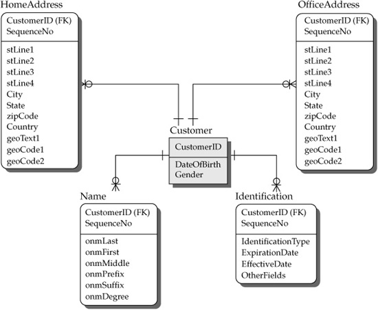
6. Create an MDM-Star schema. In the MDM world, an MDM-Star schema is a natural representation of the concept of a master entity. Figure 7-5 represents an MDM-Star with an entity Customer that can have multiple names, multiple addresses, and multiple pieces of identification. Relatively few attributes have a one-to-one relationship to the center of the star Customer (examples include Date of Birth and Gender).

In the previous paragraph we introduced a new term: “MDM-Star.” Indeed, instead of being presented as a single entity box in a typical relational model, the model in Figure 7-5 represents a master entity, Customer, as an MDM-Star with the customer identifier in the center of the star and the attributes hanging around the center with one-to-many relationships between the CustomerID and each of the attributes. The direction of one-to-many relationships from the center of the star to the attributes makes the MDM-Star look different from a data warehousing star schema structure, where one-to-many relationships are directed from the dimensions to the center of the star (fact table). Despite that, the MDM-Star possesses the same benefits as the traditional data warehousing star schema design. The MDM-Star schema design is optimized for entity resolution and relationship resolution, and supports very high performance for search, matching, and linking for millions and even billions of records. Figure 7-5 depicts only one star representing one entity: Customer. Similarly, an MDM-Star should be created for each MDM entity that requires algorithmic entity resolution or relationship resolution.

Identification in Figure 7-5 represents pieces of identification such as Social Security Number, Driver’s License, Passport, and so on.

The MDM-Star design is not optimized for complex cross–MDM-Star analytical queries. Applications modeled with the MDM-Star modeling style provide cross-entity navigation functionality through relationships, which typically meets the operational needs of MDM Data Hub users.

FIGURE 7-5 An MDM-Star for a single entity (Customer)

It is appropriate to mention that the Small World theory can be applied to the MDM-Star model to evaluate its readability the way we did earlier in this chapter for the data warehouse star schema design. For an MDM-Star schema with N attributes, we can define the following:

• Order = N+1 (N attributes plus the center of the star table).

• Size = N (the number of connections between the center of the star and the attributes).

• Average Distance → 2 when the number of attributes is high (N → ∞).

• Maximum Distance = 2 (between any two attributes).

7. Model relationships. The MDM-Star design enables the modeler to create relationships. Relationships in the MDM-Star design are allowed only between the centers of the stars. Figure 7-6 represents four entities (Individual, Account, Household, and Organization) with a few relationships supported as relationship tables.

Potentially some other relationships can be defined in Figure 7-6 (for example, a relationship between an Individual and Household).

The notion of a relationship in the entity resolution and relationship resolution world is richer than that in the traditional relational world (3NF or data warehouse star schema). In the relationship resolution process, it is important to know how a relationship is created and maintained. In the traditional logical data modeling, the modeler defines a relationship by its cardinality and ordinality (in this context, ordinality refers to the order of records or some of its attributes). In the physical data model, this translates into the foreign key and primary key constraints. For example, if two entities—Brand and Product—are related by a one-to-many relationship, the physical model tells us that the foreign key (BrandID) defines a relationship between Brand and Product. The model does not tell us how this foreign key, and therefore the relationship, is created and maintained.

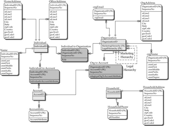
FIGURE 7-6 Illustrative MDM-star schema with multiple entities and relationships

In contrast to that, the MDM Data Hub software can algorithmically resolve relationships by applying deterministic, probabilistic, or fuzzy logic to a set of attributes responsible for a relationship; for example, the attribute “Employer” in the entity “Individual” can trigger a resolution of a relationship between the “Individual” and the “Organization.”

As we can see, this consideration is similar to what we discussed earlier in this chapter for the notion of entity resolution and how the primary keys are defined or inferred.

At a high level there exist three methods for relationship resolution, and ideally an MDM-Star model should support some or all of them even though at present traditional data modeling tools do not support such functionality:

• A relationship resolved as an exact match A foreign key constraint is an example of this relationship. The relationships in this category are resolved based on the rule that an attribute value or a key value in one entity is exactly equal to an attribute value or a key value in another entity. The value can be represented by a complex data type and composite key.

• A relationship resolved by an advanced algorithm When we discussed entity resolution, we touched upon advanced algorithms (fuzzy, probabilistic, learning algorithms). A similar approach can be applied to relationship resolution.
These algorithms resolve relationships by linking entities. The goal of the algorithm in this scenario is not to determine that two or more records represent the same entity, but rather to determine or infer relationships.
For instance, a relationship between a customer and an organization or between a customer and a household can be inferred. A Person of Interest can be related algorithmically to a terrorist network, and so on.

• A relationship defined by a human Even though advanced entity and relationship resolution algorithms can demonstrate quasi-human intelligence, it is a common requirement that an end user can override an algorithmically derived or inferred relationship. This includes the ability to create a new relationship that has not been established algorithmically or to unlink two entities that the algorithm linked to create a relationship. For example, a human resource manager can define a relationship between several employees based on a set of common interests (for example, a running club).

Oftentimes, all three methods are used in combination to accomplish the best results.

8. Model hierarchies. A hierarchy is a special case of relationships. We started discussing hierarchies in Chapters 5 and 6, and provide additional considerations of hierarchies in the context of master data modeling in this section. To recap, in the context of MDM we can define a hierarchy as an arrangement of entities (parties, accounts, products, cost centers, and so on) where entities are viewed in relationship to each other as “parents,” “children,” or “siblings/peers” of other entities according to a certain classification schema, thus forming a conceptual tree structure where all leaf nodes in the hierarchy tree can be rolled into a single “root.” Further, each hierarchy has one and only one root node. Each hierarchy node can have zero, one, or many children nodes. Each node other than the root node has one and only one parent. A hierarchy can have an unlimited number of layers.

In the MDM world, corporate hierarchies are especially important. Risk management organizations and marketing departments need to understand the corporate hierarchies of their prospects and clients to manage relationship risks and credit risks as well as to improve the intelligence of marketing and marketing outcomes. A number of vendors offer corporate hierarchy data (Dun & Bradstreet, Equifax, and so on). These hierarchies are used to resolve hierarchical relationships. This resolution follows the three methods outlined earlier where we discussed relationships. It is particularly important in Master Data Management to be able to support multiple hierarchies required by different functions in the enterprise (sales hierarchy, legal hierarchy, marketing hierarchy, and so on). Two hierarchies are shown in Figure 7-6 as illustrative examples (legal and marketing). The need for hierarchies is not limited to organizational hierarchies. For instance, employees of a company are organized in hierarchies that show reporting relationships. Product hierarchy representation is a convenient way to see a breakdown structure of complex products or bills of materials. Geographies can also be organized in hierarchies for sales territory management.

9. Define and model reference data. This step concentrates on the modeling of reference data. Reference data processes include the following:

• A definition of reference data entities (for example, Account Type, Brand, Gender, Country, and Territory).

• A definition of the lists of allowed or accepted values recognized by the enterprise across multiple functions for the reference data entities selected in the first bullet. These are typically the entities with lower record counts, ranging from very few allowed values (for example, Gender) to a few hundred records (such as Territory codes). At the same time, it is not unusual to find reference data files that are much larger; for example, a financial services securities master can contain thousands of records. And, of course, a customer or account reference file can have millions of records, where the records contain externally or internally established identifiers such as customer ID, account numbers, and so on. Regardless of the size of the reference data, managing these entities is based on the idea that only certain distinct values are allowed from the business process and data governance perspectives. The business and data governance organization working together define the distinct values that should be allowed for the reference data.

• A definition of standards and formats that the attributes and list values must comply with. Definitions of standards can apply to short lists of allowed values and the entities with very high distinct value counts, such as social security number, phone number, and e-mail address. Account numbers and credit card numbers also follow specific formats that must be validated. This type of validation is one of the data governance functions.

The model presented in Figure 7-6 is easily readable. Given that a mature enterprise may have hundreds of reference data entities and rules, their inclusion in the diagram in Figure 7-6 would hamper the model readability. This issue can be addressed by using multiple views of the MDM canonical (systems- and applications-agnostic) data model. Different views should be able to turn on or off the display of the reference data. The existing data modeling tools do not adequately support this type of data modeling need.

10. Map the model to source systems and define the source systems’ entities and attributes that will be stored in the MDM Data Hub. So far, we have been focusing our data modeling steps on the development of master data structures for the canonical master data model, which is independent of operational source systems. Typically an MDM Data Hub redundantly stores the source system data used in the process of matching, linking, and entity/relationship resolution to infer master entity records and relationships. Early versions of MDM Data Hub products made some attempts not to store the source system records in the MDM Data Hub redundantly, but rather access the source system records directly in the source systems. This type of federated architecture has not been adopted in the field due to performance problems. Therefore, the modeler should be able to model a representation of data where the model explicitly shows which systems, tables, and attributes contribute to the attributes in the canonical MDM-Star model depicted in Figure 7-6.

Figure 7-7 provides the source system–specific view of the MDM-star schema presented in Figure 7-6.

Let’s analyze the differences between the canonical (system-agnostic) representation in Figure 7-6 and the system-specific model representation in Figure 7-7:

• Figure 7-7 shows that the centers of the stars for the source-specific models have additional identifiers: the identifier that shows which system each record is originated from (SystemID) and the system-specific identifiers for the record (SystemCustomerID, SystemAccoutID, SystemOrganizationID, and SystemProductID). This model is more granular than the one in Figure 7-6 and allows more than one source system record to contribute to the canonical master entity representation (system-agnostic) depicted in Figure 7-6.

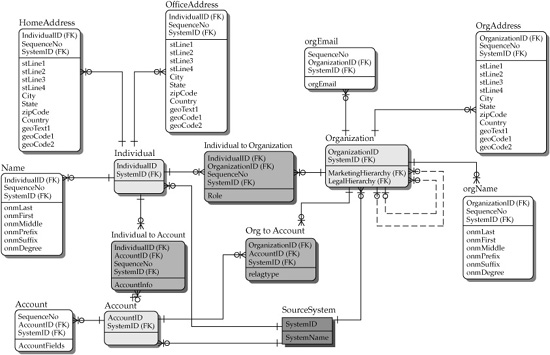
FIGURE 7-7 An illustrative MDM-Star schema (source-specific representation)

Another significant difference between Figures 7-6 and 7-7 is that Figure 7-6 contains four MDM-Stars, whereas Figure 7-7 displays only three MDM-Stars. Figure 7-8 explains the reason for this. The Individual MDM-Star in the source-specific model yields two entities: Individual and Household. The entity Customer in Figure 7-6 is obtained by entity resolution that takes into account all of a person’s identity attributes, and the entity Household is obtained from Household identity attributes. The Household identity attributes do not include attributes such as First Name, Social Security Number, and any other attributes of an individual Customer.

The way the source system attributes can contribute to the values of the canonical entity attributes is by following the attribute survivorship rules that we will discuss in more detail in Part IV. Ideally, it would be great to keep these attribute survivorship rules in a data modeling tool. Unfortunately, many existing data modeling tools do not present a convenient way of doing this.

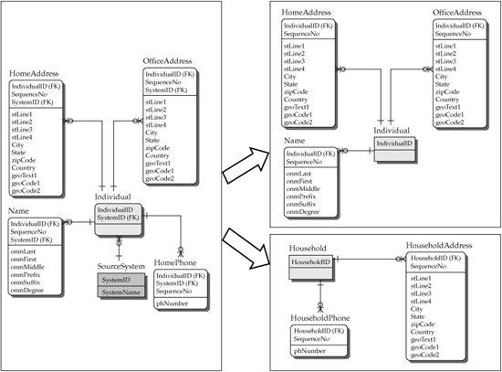
FIGURE 7-8 Mapping between the canonical model and a source-specific model

It should be noted that the MDM-Star system-specific structures in Figure 7-7 are so efficient from the entity resolution and relationship resolution perspectives that the canonical model in Figure 7-6 (system agnostic) may not even be persisted but rather created dynamically. This design is proven to support use cases with many millions of records. In Part IV, we will discuss the pros and cons of having the canonical-level record persisted in the MDM Data Hub versus the solution where the canonical-level record is retrieved dynamically.

Reference code reconciliation is an important part of reference data mapping. The reference codes, allowed values, and standards defined in the reference data section must be mapped to the values and codes used in the source systems. It is an architectural decision which component is responsible for reference code reconciliation semantics. This can be done inside the Data Hub or by an external component.

To a significant extent the data governance organization decides which reference codes, values, and standards have enterprise significance and which enumerations, codes, and standards should be managed in specific functional areas. We will discuss the issues of data governance in more detail in Part IV.

From the Master Data Management perspective, third-party data sources that help resolve entities and relationships and enrich data should also be considered as data sources and their attributes modeled in the source-specific schema. Third-party data sources are typically considered trusted master data sources. This means that the third-party records cannot be linked by a single enterprise identifier, unlike the internal enterprise records residing in operational systems.

11. Model landing and staging areas. Landing and staging area data models are often used to load the data into the Data Hub (refer to the Data Zone architecture discussion in Chapter 5 for additional details on these areas). There is a trend to make these areas less significant, especially when real-time integration between the source systems and the MDM Data Hub is required. The source system record is sent to the MDM Data Hub through an Enterprise Service Bus (ESB). Modern MDM Data Hub products support a set of services to transform the data and present the canonical data correctly and dynamically (Figure 7-6), even if the records are not perfectly cleansed in the system-specific layer (Figure 7-7).

12. Model for master data consumption, including data warehousing dimensions. The MDM-Star model optimized for entity resolution, relationship resolution, and entity-specific searches, with the need to find a particular customer, product, location, and so on, is not optimized for other types of queries. For instance, queries that require joins of multiple MDM-Star entities are not efficient. The relationships between the centers of the MDM-Stars are typically used to navigate between the MDM-Stars rather than for the queries that execute multientity MDM-star joins.

Consequently, there is a need for a model or models optimized for multientity joins. This can include operational data stores and data warehouses. A variety of industry-specific model libraries exist that can be leveraged as a starting point for developing operational data stores and data warehouses. Some examples of these libraries include:

• IBM Insurance Information Warehouse ⁹

• Libraries of industry models developed by Len Silverston ^10,11,12

• Insurance models developed by Prima Solutions ¹³

• Oracle industry data models ¹⁴

• ESRI data models ¹⁵

At the time of this writing, many MDM Data Hub products offer limited support for integration with industry-standard models. This fact is also an opportunity for MDM vendors to enhance their MDM Data Hub products to support industry-standard data models in future releases.

To further illustrate MDM data modeling requirements let’s focus on the needs of the analytical MDM. We can view the analytical MDM as a separate class of consuming applications that implement some standard architectural patterns. One highly important pattern of the analytical MDM is the ability of the MDM Data Hub to create and maintain the content of data warehousing dimensions. An important question comes up as to what extent MDM should be responsible for the creation and maintenance of master data in the traditional data warehousing formats required for dimensional modeling and support for slowly changing dimensions. Figures 7-9 depicts a scenario where source systems feed a data warehouse.

The data warehouse is used to consolidate, standardize, and conform dimensional information as well as to bring the dimensional data into the required data warehousing formats used to support slowly changing dimension and other data warehousing requirements. The data warehouse is also responsible for storing and managing the fact data.

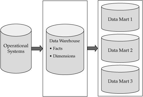
FIGURE 7-9 Data warehousing data flow in the absence of MDM

In a typical data warehouse–data mart scenario, subsets of facts and dimensions are fed into data marts that are used for reporting and analytics. It is important to understand that as a common best practice, the data warehouse is not used for reporting and analytics directly.

An MDM Data Hub can be used to manage data warehousing dimensions, as shown in Figure 7-10.

The architectural change that resulted from the introduction of an MDM Data Hub is illustrated by a comparison of Figures 7-9 and 7-10. Figure 7-10 shows that the data warehouse is no longer managing dimensional data but rather only the fact data and dimensional keys. The ownership of dimension management, including key functionality of dimensional hierarchy management, has moved to the Data Hub.

Let’s discuss the nature of the changes required to translate the MDM-Star structures into a data warehousing format supporting slowly changing dimensions.

As we discussed earlier in this chapter, every change in the MDM-Star applied at the source system level is translated into the canonical-level structure. From the dimensional modeling perspective, it is important to capture dimensional snapshots within certain time intervals (for example, daily). If multiple changes occur during a day, intermediate daily changes are not captured in the dimensional world. The effective dates for the changes to take effect must be calculated for both versions of the record.

Specifically, prior to the change, only a one dimensional record exists: version 1. The record is Active before the change, and the start date shows the date when the record was originally created, whereas the end date (01/01/9999) signifies some unknown date in the future. After the change, version 1 of the record becomes Inactive, and the end date is set to the date when the change occurred (02/19/2010). The new record is created (version 2) and becomes Active with the new start date (02/20/2010) and the end date (01/01/9999). This type of transition requires a process that identifies the records changed over a predefined period (for example, a business day), deactivates the updated version, and creates the new active version as described in this paragraph.

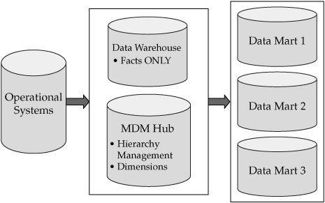
FIGURE 7-10 Data warehousing data flow after an MDM implementation

Data Modeling Styles and Their Support for Multidomain MDM

Early MDM implementations primarily focused on a single MDM domain: most frequently Party or Product. As MDM adoption continues to grow across all industry segments, other domains have proven to be important: Location, Service, Asset, and so on. It is important to take into the account the fact that in addition to the significant commonalities of data modeling features for each of the named domains across industries, there are also some significant differences specific to industries and enterprises. For instance, the Party model for Person of Interest supporting law enforcement can differ significantly from the Party model required for a retail store. Both models may differ from what is required to support wealth management organization needs. Similarly, in the product domain, financial services products differ significantly from manufacturing products, which can translate into significant differences in the required data models. It should be noted that even if an MDM data model meets the original requirements at the MDM program initiation, the model may not be able to meet evolving MDM requirements. If an MDM initiative started with one or two domains originally defined by business requirements, other domains may become priorities of the future implementation phases. Generally speaking, this discussion focuses on the need for flexibility of the data model required to support multiple domains, functional areas, entities, attributes, relationships, and evolving business requirements.

This flexibility should be built into the model while at the same time retaining robustness, support for performance, and the maintainability of the MDM Data Hub.

Each of the data modeling styles can and should be implemented using the service-oriented architecture (SOA). The nature of the services and their granularity, to a significant extent, depend on the data modeling style.

Figure 7-11 depicts the primary MDM data modeling styles used by MDM vendors. Understanding these styles is important and may drive the selection of the MDM product and vendor.

These modeling styles differ by the degree of model abstraction and flexibility to support a variety of data modeling requirements.

• Approach 1: The “Right” Data Model

• Approach 2: Metadata Model

• Approach 3: Abstract MDM-Star Model

Approach 1: The “Right” Data Model

The first of the data modeling styles (on the left in Figure 7-11) approaches the data model with a specific data domain or domains in mind. For example, if the model concentrates on the Party domain, the model would typically include database objects (tables) such as Party, Customer, or Contact with the corresponding primary key (PartyID, CustomerID, or ContactID). Such a model is not intended to support the product domain. Many business domain–specific products were originally focused on a single domain. If a customer has acquired an MDM Data Hub product supporting only the Party domain, the need for the Product, Location, or Asset domain would drive the need for another MDM product. There are a number of disadvantages in having multiple products supporting different MDM data domains including costs, the needs to deal with potentially overlapping data modeling areas and functions offered by different MDM products, and the resulting needs to extend governance and integration efforts. To address these shortcomings, domain model–specific MDM products have evolved by supporting and integrating additional data domain areas (for example, adding and integrating the product domain to the party data model). The data domain model integration is a key because, oftentimes, data domain–specific products grew not organically but through the acquisitions of the MDM Data Hub products supporting different data domains.

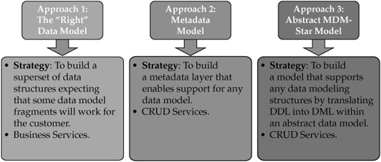
FIGURE 7-11 Master data modeling styles

Approach 2: Metadata Model

The second MDM data modeling style (in the middle in Figure 7-11) does not persist any data structures (tables) “out of the box.” Data tables are defined in a metadata layer for each MDM project as needed. The flexibility of such metadata-driven MDM products allows the MDM modelers and architects to build multidomain MDM products and apply on-going changes to the composite data model. Clearly, this approach requires complex metadata management because the physical data model may not comply with the MDM-Star modeling rules. Consequently, the metadata should be able to map attributes from multiple tables that comprise a logical MDM entity. The complexity of this design may make it difficult to resolve errors in the metadata, which affects the ease of maintenance of the product. The overall performance of the product designed this way may suffer from the need to perform multiple table joins even within a single data domain or entity. This performance problem grows with the number of data domain records and can cause significant difficulties if entity resolution for millions of records is required.

Approach 3: Abstract MDM-Star Model

The third data modeling style is an abstracted MDM-Star model. This data modeling style converts the typical SQL Data Definition Language (DDL) constructs such as entity names and primary key definitions into the constructs of the SQL Data Manipulation Language (DML). For instance, all entity names (Product, Customer, Broker, Service, Asset, Account, and so on) are stored as rows in a dedicated database table. The primary keys (ProductID, CustomerID, BrokerID, ServiceID, AccountID, and so on) are stored in a separate table, too. The association between the entity name and the primary key is resolved by storing the entity identifier on the record. Such a record, for the canonical-level model, may include the primary key and the key identifying the entity the primary key belongs to. The source-specific level of the model, in addition, holds the system identifier. This master data modeling style is optimized for entity and relationship resolution and can be used for an unlimited number of data domains and entities within the MDM-Star modeling style.

Because physical table names and attribute names are abstracted, the data model would not display the names like Product, Customer, and so on, which complicates the readability of the model. Business analysts would have to deal with the business services or data services layer to understand the model and its scope from the data domain perspective. As an alternative, MDM-Star abstracted models require additional components known as “bridges.”¹⁶ Such a bridge enables the product to integrate with many data modeling and database designer tools and display the abstracted model as a traditional Entity Relational Diagram (ERD).

We started this chapter with an overview of the predominant data modeling patterns. We used these patterns to describe a variety of MDM needs and translate these needs into a number of data modeling structures and components that must be maintained with properly architected redundancy. Our goal was to make it clear why a widely accepted data modeling practice to limit data modeling effort by a 3NF canonical model is not sufficient to address the complexity of Master Data Modeling needs. As data warehousing modeling techniques evolved in the 1990s and continued to evolve in the last decade, we can see the beginning of a similar data modeling trend for master data modeling in recent years, and we see that master data modeling is growing as a separate specialized data modeling discipline. This fact is often underestimated by the data modelers assigned to MDM initiatives.

We have discussed and defined the process of master data modeling and explained each of the data modeling steps along with why these steps are required and what makes them and master data modeling in general different from OLAP and OLTP. We have concluded with a discussion of three primary approaches used by the MDM Data Hub product vendors, and offered a comparison of these data modeling design approaches by highlighting their strengths, weaknesses, and areas of focus. As we could see, different MDM vendors concentrate on different types of data models and data modeling abstraction layers.

The data modeling “philosophy” with which an MDM Data Hub is built drives significant differences in the structure, the level of granularity of services, and the functionality and performance offered by the MDM Data Hub products.

References

1. Codd, E.F. (June 1970). “A Relational Model of Data for Large Shared Data Banks.” Communications of the ACM 13 (6): 377–387.

2. Codd, E.F. “Further Normalization of the Data Base Relational Model.” (Presented at Courant Computer Science Symposia Series 6, “Data Base Systems,” New York City, May 24–25, 1971.) IBM Research Report RJ909 (August 31, 1971). Republished in Data Base Systems: Courant Computer Science Symposia Series 6 (Randall J. Rustin, Editor). Prentice-Hall (1972).

3. Codd, E.F. “Recent Investigations into Relational Data Base Systems.” IBM Research Report RJ1385 (April 23, 1974). Republished in Proc. 1974 Congress (Stockholm, Sweden, 1974). North-Holland (1974).

4. Hillard, Robert. “Small Worlds.” http://mike2.openmethodology.org/index.php/Small_Worlds_Data_Transformation_Measure.

5. Fagin, Ronald. “Multivalued Dependencies and a New Normal Form for Relational Databases.” ACM Transactions on Database Systems 2 (1): 267. September 1977. http://www.almaden.ibm.com/cs/people/fagin/tods77.pdf.

6. Kent, William. “A Simple Guide to Five Normal Forms in Relational Database Theory,” Communications of the ACM, (1983) 26: 120–125.

7. Kimball, Ralph. The Data Warehouse Toolkit: Practical Techniques for Building Dimensional Data Warehouses. Wiley (1996). 162.

8. Linstedt, Dan E. “Data Vault Series 1—Data Vault Overview.” July 1, 2002. http://www.tdan.com/view-articles/5054/.

9. http://www-01.ibm.com/software/data/industry-models/insurance-data/.

10. Silverston, Len. The Data Model Resource Book, Revised Edition, Vol. 1: A Library of Universal Data Models For All Enterprises. Wiley Computer Publishing (March 2001).

11. Silverston, Len. The Data Model Resource Book, Revised Edition, Vol. 2: A Library of Universal Data Models For Specific Industries. Wiley Computer Publishing (March 2001).

12. Silverston, Len and Angew, Paul. The Data Model Resource Book, Vol. 3: Universal Patterns for Data Modeling. Wiley Computer Publishing (January 2009).

13. http://www.prima-solutions.com/frontOffice/produits/primaIBCS.jsp?gclid= CObu3e7ug6ACFVl35QodXlsYvQ.

14. http://blogs.oracle.com/datawarehousing/2009/04/oracle_releases_industry_ data.html.

15. http://support.esri.com/index.cfm?fa=downloads.datamodels.gateway.

16. http://www.metaintegration.net/Products/MIMB/OMGXMI.html.