
Description of the Solution of Equations
One of the most fundamental problems in scientific computing is solving equations of the form f (x) = 0. This is often referred to as finding the roots, or zeros, of f (x). Here, we are interested in the real roots of f (x), as opposed to any complex roots it might have. Specifically, we will focus on finding real roots when f (x) is a polynomial.
Finding Roots with Newton’s Method
Although factoring and applying formulas are simple ways to determine the roots of polynomial equations, a great majority of the time polynomials are of a large enough degree and sufficiently complicated that we must turn to some method of approximation. One of the best approaches is Newton’s method. Fundamentally, Newton’s method looks for a root of f (x) by moving closer and closer to it through a series of iterations. We begin by choosing an initial value x = x 0 that we think is near the root we are interested in. Then, we iterate using the formula:
until xi + 1 is a satisfactory approximation. In this formula, f (x) is the polynomial for which we are trying to find a root, and f ' (x) is the derivative of f (x).
Computing the Derivative of a Polynomial
The derivative of a function is fundamental to calculus and can be described in many ways. For now, let’s simply look at a formulaic description, specifically for polynomials. To compute the derivative of a polynomial, we apply to each of its terms one of two formulas:
where k is a constant, r is a rational number, and x is an unknown. The symbol d /dx means “derivative of,” where x is the variable in the polynomial. For each term that is a constant, we apply the first formula; otherwise, we apply the second. For example, suppose we have the function:
In order to compute f ' (x), the derivative of f (x), we apply the second formula to the first three terms of the polynomial, and the first formula to the last term, as follows:
Sometimes it is necessary to compute higher-order derivatives as well, which are derivatives of derivatives. For example, the second derivative of f (x), written f '' (x), is the derivative of f ' (x). Similarly, the third derivative of f (x), written f ''' (x), is the derivative of f '' (x), and so forth. Thus, to compute the second derivative of f (x) in the previous equation, we compute the derivative of f ' (x), as follows:
Understanding the First and Second Derivative
Now let’s look at what derivatives really mean. To use Newton’s method properly, it is important to understand the meaning of the first and second derivative in particular.
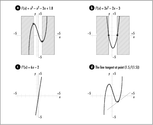
The value of the first derivative of f (x) at some point x = x 0 indicates the slope of f (x) at point x 0; that is, whether f (x) is increasing (sloping upward from left to right) or decreasing (sloping downward). If the value of the derivative is positive, f (x) is increasing; if the value is negative, f (x) is decreasing; if the value is zero, f (x) is neither increasing nor decreasing. The magnitude of the value indicates how fast f (x) is increasing or decreasing. For example, Figure 13.6, example a, depicts a function whose value increases within the shaded regions; thus, these are the regions where the first derivative is positive. The plot of the first derivative crosses the x-axis at the points where the slope of f (x) changes sign.
The value of the second derivative of f (x) at some point x = x 0 indicates the concavity of f (x) at point x 0, that is, whether the function is opening upward or downward. The magnitude of the value indicates how extreme the concavity is. In Figures 13-6a and 13-6c, the dotted line indicates the point at which the concavity of the function changes sign. This is the point at which the plot of the second derivative crosses the x-axis.
Another way to think of the value of the derivative of f (x) at some point x = c is as the slope of the line tangent to f (x) at c, expressed in point-slope form. The point-slope form of a line is:
Thus, if f (x) = x 3 - x 2 - 3x + 1.8 as shown in Figure 13.6, example a, the equation of the line tangent to f (x) at c = 1.5 as can be determined as follows. Figure 13.6, example d, is a plot of this line along with f (x).
Selecting an Initial Point for Newton’s Method
Now that we understand a little about derivatives, let’s return to Newton’s method. Paramount to Newton’s method is the proper selection of an initial iteration point x 0. In order for Newton’s method to converge to the root we are looking for, the initial iteration point must be “near enough” and on the correct side of the root we are seeking. There are two rules that must be followed to achieve this:
Determine an interval [a, b ] for x 0 where one and only one root exists. To do this, choose a and b so that the signs of f (a) and f (b) are not the same and f ' (x) does not change sign. If f (a) and f (b) have different signs, the interval contains at least one root. If the sign of f ' (x) does not change on [a, b ], the interval contains only one root because the function can only increase or decrease on the interval.
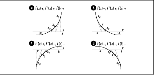
Choose either x 0 = a or x 0 = b so that f (x 0) has the same sign as f '' (x) on the interval [a, b ]. This also implies that f '' (x) does not change sign on the interval. Recall that the second derivative of f (x) is an indication of concavity. If f '' (x) does not change sign and x 0 is chosen so that f (x 0) has the same sign as f '' (x), each successive iteration of Newton’s method will converge closer to the root on the interval [a, b ] (see Figure 13.7).
In each of the four parts of Figure 13.7, f (x) is shown as a heavy line, and a and b are shown as vertical dotted lines. If f (a) matches the criteria just given, iteration begins at a and tangent lines slope from a toward the root to which we would like to converge. If f (b) matches the criteria above, iteration begins at b and tangent lines slope from b toward the root to which we would like to converge.
How Newton’s Method Works
As an example, suppose we would like to find the roots of f (x) = x 3 - x 2 - 3x + 1.8. Figure 13-8 illustrates that this function appears to have three roots: one on the interval [-2, -1], another on the interval [0, -1], and a third on the interval [2, 3]. Once we have an idea of the number and location of a function’s roots, we test each interval against the rules for selecting an initial iteration point. To do this, we need to know the following:
Using this information, we see that the interval [-2, -1] satisfies the first rule because f (-2) = -4.2 and f (-1) = 2.8, and f ' (x) does not change sign on the interval: it is always positive. Considering this, we know there is, in fact, one and only one root on the interval [-2, -1]. To satisfy the second rule, we see that f '' (x) does not change sign on the interval: it is negative. We select x 0 = -2 as the initial iteration point since f (-2) = -4.2 is also negative. Figure 13.8 illustrates calculating the root on this interval to within 0.0001 of its actual value. We end up iterating five times to obtain this approximation.
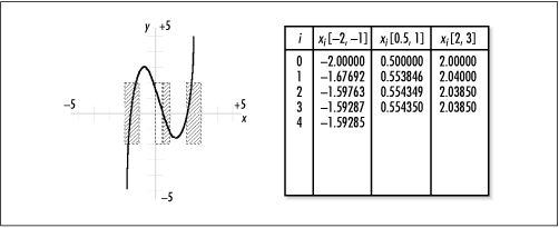
Moving to the root on the interval [0, 1], we see that the first rule is satisfied just as for the previous interval. However, the sign of f '' (x) is not constant on this interval; therefore, the interval does not satisfy the second rule. Suspecting that the root is closer to 1 than 0, we try the interval [0.5, 1] next, which corrects the problem. The first rule is satisfied because f (0.5) = 0.175 and f (1) = -1.2, and f ' (x) does not change sign on the interval: it is negative. To complete the second rule, we select x 0 = 0.5 since f (0.5) = 0.175 is positive and has the same sign as f '' (x) over the interval [0.5, 1]. Figure 13.8 illustrates calculating the root on this interval to within 0.0001 of its actual value. We end up iterating four times to obtain this approximation. Calculating the third root proceeds in a similar manner.