12
Dynamic Behavior of Nanobeam Using Strain Gradient Model
Subrat Kumar Jena, Rajarama Mohan Jena, and Snehashish Chakraverty
Department of Mathematics, National Institute of Technology Rourkela, Rourkela, Odisha, 769008, India
12.1 Introduction
Dynamic analysis of nanostructures is very crucial for engineering design of several electromechanical devices such as nanoprobes, nanooscillators, nanosensors, etc. This analysis is very fundamental as the experimental study in nanoscale is very tedious and expensive. Also, classical mechanics fails to address the nanoscale effect. In this regard, several nonclassical theories have been introduced by researchers to address the small‐scale effect. These theories include strain gradient theory [1], couple stress theory [2], modified couple stress theory [3], micropolar theory, and nonlocal elasticity theory [4]. Investigations related to the dynamical analysis of beams, membranes, nanobeams, nanotubes, nanoribbons, etc., are reported in the literature [5–14].
Akgöz and Civalek [15] analytically studied the static behavior of the Euler–Bernoulli nanobeam under the framework of the modified strain gradient theory and modified couple stress theory. They also investigated the influence of size effect and material parameters on the static response of the beam. Akgöz and Civalek [16] again developed a size‐dependent higher order shear deformation beam using modified strain gradient theory, which can address both the microstructural and shear deformation effects. The dynamical behavior is studied analytically using Navier solution. The static and dynamic analyses of size‐dependent functionally graded microbeams under the framework of Timoshenko beam theory and strain gradient theory are reported in Ansari et al. [17,18]. Kahrobaiyan et al. [19] studied the static and dynamic behaviors of size‐dependent functionally graded simply supported Euler–Bernoulli microbeams using strain gradient theory. Generalized differential quadrature method has been employed by Khaniki and Hosseini‐Hashemi [20] to analyze the buckling behavior of tapered nanobeams using nonlocal strain gradient theory for simply supported boundary condition. Free vibration of a size‐dependent functionally graded Timoshenko beam is studied analytically by Li et al. [21] using strain gradient model implementing Navier's solution. Li et al. [22] again investigated the longitudinal vibration of the nonlocal strain gradient rod by using an analytical method as well as the finite element method. Wave propagation for Euler–Bernoulli beams has been presented by Lim et al. [23] using higher order nonlocal theory as well as strain gradient theory. Some other studies of strain gradient model are also reported in the literature [24–27].
As per the title of the chapter, the dynamical behavior of, in particular, free vibration of Euler–Bernoulli strain gradient nanobeam is investigated using the differential transform method (DTM) for SS and CC boundary conditions. Validation and convergence study of the frequency parameters of strain gradient nanobeam are also conducted. Further, the effects of small‐scale parameters and length‐scale parameters on frequency parameters are reported for the first four modes of frequency parameters through graphical and tabular results.
12.2 Mathematical Formulation of the Proposed Model
The equation of motion of Euler–Bernoulli nanobeam can be expressed as [20]
where M is the bending moment that is defined as ![]() , P is the applied compressive force due to mechanical loading, ρ is the mass density, and A is the area of cross section of the beam. For an isotropic beam, the first‐order strain gradient model can be written as [20,23,24]
, P is the applied compressive force due to mechanical loading, ρ is the mass density, and A is the area of cross section of the beam. For an isotropic beam, the first‐order strain gradient model can be written as [20,23,24]

where σxx is the normal stress, E is Young's modulus, εxx is the classical strain, e0a is the nonlocal parameter, and l is the length‐scale parameter. Now, multiplying Eq. (12.2) by z dA and integrating over the area, we may get
Plugging Eq. (12.1) in Eq. (12.3), the nonlocal bending moment may be written as

Inserting Eq. (12.4) in the equation of motion of beam, i.e. Eq. (12.1), the governing equation can be obtained as

Now assuming the equation of motion as sinusoidal, viz., w(x, t) = w0(x)eiωt, Eq. (12.5) can be rewritten as

Let us consider the following dimensionless parameters as
Using the above dimensionless parameters in Eq. (12.6), the nondimensional form of governing equation can be expressed as

Now by letting ![]() in Eq. (12.7), the nondimensional form of transverse vibration equation of nonlocal strain gradient beam can be reduced to
in Eq. (12.7), the nondimensional form of transverse vibration equation of nonlocal strain gradient beam can be reduced to

12.3 Review of the Differential Transform Method (DTM)
DTM is a semianalytical technique that was first introduced by Zhou [28] for solving linear and nonlinear initial value problems arising in electrical circuits. Since then, this technique has been used in many problems arising in different fields of science and engineering. Use of DTM in structural dynamics problem can be found in Chen and Ho [29], Ayaz [30], Ayaz [31], Ozdemir and Kaya [32], Ozdemir and Kaya [33], Balkaya et al. [34], Ozgumus and Kaya [35], Zarepour et al. [36], and Nourifar et al. [37].
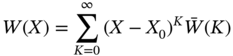
Let us consider an analytic function W(X) in a domain D and assume that X = X0 be any point in that domain. Then, the function W(X) can be expressed by a power series having a center located at X0. The differential transform of the function W(X) can be written as

where W(X) is the original function and ![]() is the transformed function. The inverse differential transformation is defined as
is the transformed function. The inverse differential transformation is defined as
Combining Eqs. (12.9) and (12.10), we obtain

The function W(X) can be expressed by a finite series, and therefore, Eq. (12.11) can be written as

Implementation of differential transform on some basic functions and the boundary conditions are depicted in Tables 12.1–12.2.
Table 12.1 Implementation of DTM on some basic functions [36].
| Original function | Transformed function |
| W(X) = W1(X) ± W2(X) | |
| W(X) = αW1(X) | |
| W(X) = W1(X) W2(X) | 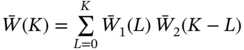 |
 |
|
| W(X) = eαX |
Table 12.2 Implementation of DTM on boundary conditions [36].
| X = 0 | X = 1 | ||
| Original B.C. | Transformed B.C. | Original B.C. | Transformed B.C. |
| W(0) = 0 | W(1) = 0 | ||
 |
 |
||
 |
 |
||
 |
 |
||
12.4 Application of DTM on Dynamic Behavior Analysis
In this section, we will formulate and discuss the dynamic behavior of in particular vibration characteristics of strain gradient nanobeam using DTM to find frequency parameters. Implementing DTM and referring to Table 12.1, the nondimensional form of transverse vibration equation of nonlocal strain gradient beam, i.e. Eq. (12.8), is now reduced into

Now rearranging Eq. (12.13), we obtain the recurrence relation as

Referring to Table 12.2, the simply supported‐simply supported (SS) boundary condition is given as
At X = 0:
At X = 1:


Substituting the values of ![]() from Eq. (12.15), into therecurrence relation Eq. (12.14), we obtain
from Eq. (12.15), into therecurrence relation Eq. (12.14), we obtain

where C1, C2, and C3 are constants. Substituting all the above values of ![]() in Eqs. (12.16), (12.17), and (12.18), we will get the system of equations in matrix form as
in Eqs. (12.16), (12.17), and (12.18), we will get the system of equations in matrix form as

where ![]() , i, j = 1, 2, 3. are the polynomials of λ corresponding to the number of terms as N.
, i, j = 1, 2, 3. are the polynomials of λ corresponding to the number of terms as N.
As C1 ≠ 0, C2 ≠ 0, and C3 ≠ 0, Eq. (12.19) implies

Now by solving Eq. (12.20), we get ![]() , where i = 1, 2, 3, …N and
, where i = 1, 2, 3, …N and ![]() is the ith mode frequency parameter corresponding to the term N. The value of N for the convergence of the frequency parameter can be obtained from the following relation
is the ith mode frequency parameter corresponding to the term N. The value of N for the convergence of the frequency parameter can be obtained from the following relation
where ![]() is the ith mode frequency corresponding to N,
is the ith mode frequency corresponding to N, ![]() is the ith mode frequency corresponding to N − 1, and ε is the degree of precision.
is the ith mode frequency corresponding to N − 1, and ε is the degree of precision.
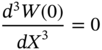
Similarly, by referring to Table 12.2, the Clamped‐Clamped (CC) boundary condition can be demonstrated as
At X = 0:
At X = 1:


Referring to the same procedures as that of SS case, we also obtain the frequency parameter for Clamped‐Clamped (CC) boundary condition.
12.5 Numerical Results and Discussion
All the computations for tabular as well as graphical results are carried out using MATLAB tailored code developed by the authors.
12.5.1 Validation and Convergence
Validation and convergence of the present results obtained by DTM are studied in this subsection through graphical as well as tabular results. Setting the length‐scale parameter “l” to zero, the strain gradient model is reduced to Eringen's nonlocal model, and the transverse vibration equation of strain gradient nanobeam, i.e. Eq. (12.8), will be converted into vibration equation for nanobeam. In this regard, β2 has been assigned zero, and the present results have been compared with other well‐known results reported in the published literature [38]. Tables 12.3 and 12.4 demonstrate the validation of present results with Wang et al. [38] for SS and CC boundary conditions, respectively. In this comparison, the first three frequency parameters ![]() are considered for validation, keeping all other parameters the same as Wang et al. [38]. From these Tables 12.3 and 12.4, we may certainly evident that the present results show admirable agreement with Wang et al. [38]. The convergence of the model is also explored through the graphical results, which are illustrated in Figures 12.1 and 12.2. Both Figures 12.1 and 12.2 represent pointwise convergence of SS and CC boundary conditions, which are plotted by taking β1 = 1 and β2 = 0.5. From the Figures 12.1 and 12.2, it is revealed that lower mode frequency requires less number of terms than that of higher mode. Approximately 35 number of terms is required for the convergence of third mode frequency of SS boundary condition, whereas 45 number of terms is required for the third mode of CC boundary condition. These figures clearly depict the convergence of the present model by DTM.
are considered for validation, keeping all other parameters the same as Wang et al. [38]. From these Tables 12.3 and 12.4, we may certainly evident that the present results show admirable agreement with Wang et al. [38]. The convergence of the model is also explored through the graphical results, which are illustrated in Figures 12.1 and 12.2. Both Figures 12.1 and 12.2 represent pointwise convergence of SS and CC boundary conditions, which are plotted by taking β1 = 1 and β2 = 0.5. From the Figures 12.1 and 12.2, it is revealed that lower mode frequency requires less number of terms than that of higher mode. Approximately 35 number of terms is required for the convergence of third mode frequency of SS boundary condition, whereas 45 number of terms is required for the third mode of CC boundary condition. These figures clearly depict the convergence of the present model by DTM.
Table 12.3 Comparison of present results with Wang et al. [38] for SS case.
| Present | Ref. [38] | |||||
| 0 | 3.1416 | 6.2832 | 9.4248 | 3.1416 | 6.2832 | 9.4248 |
| 0.1 | 3.0685 | 5.7817 | 8.0400 | 3.0685 | 5.7817 | 8.0400 |
| 0.3 | 2.6800 | 4.3013 | 5.4422 | 2.6800 | 4.3013 | 5.4422 |
| 0.5 | 2.3022 | 3.4604 | 4.2941 | 2.3022 | 3.4604 | 4.2941 |
| 0.7 | 2.0212 | 2.9585 | 3.6485 | 2.0212 | 2.9585 | 3.6485 |
Table 12.4 Comparison of present results with Wang et al. [38] for CC case.
| Present | Ref. [38] | |||||
| 0 | 4.7300 | 7.8532 | 10.9956 | 4.7300 | 7.8532 | 10.9956 |
| 0.1 | 4.5945 | 7.1402 | 9.2583 | 4.5945 | 7.1402 | 9.2583 |
| 0.3 | 3.9184 | 5.1963 | 6.2317 | 3.9184 | 5.1963 | 6.2317 |
| 0.5 | 3.3153 | 4.1561 | 4.9328 | 3.3153 | 4.1561 | 4.9328 |
| 0.7 | 2.8893 | 3.5462 | 4.1996 | 2.8893 | 3.5462 | 4.1996 |
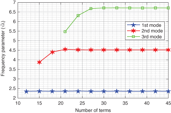
Figure 12.1 Frequency parameter vs. number of terms for SS boundary condition.

Figure 12.2 Frequency parameter vs. number of terms for CC boundary condition.
12.5.2 Effect of the Small‐Scale Parameter
The effect of small‐scale parameter on the frequency parameter has been investigated through this subsection. The values of small‐scale parameter ![]() are considered as 0, 0.5, 1, 1.5, 2, 2.5, 3, 3.5, 4, 4.5, and 5. In this regard, both the tabular and graphical results are depicted for the first four frequency parameters of SS and CC boundary conditions. Tables 12.5 and 12.6 represent the tabular results for first four frequency parameters for different small‐scale parameters. Likewise, Figures 12.3 and 12.4 demonstrate the graphical results for SS and CC boundary conditions. It is witnessed that frequency parameters decrease with the increase of small‐scale parameters for both the boundary conditions of all modes. This reduction is very high in case of higher modes than lower modes. Further, to elucidate the nonlocal effect, the response of
are considered as 0, 0.5, 1, 1.5, 2, 2.5, 3, 3.5, 4, 4.5, and 5. In this regard, both the tabular and graphical results are depicted for the first four frequency parameters of SS and CC boundary conditions. Tables 12.5 and 12.6 represent the tabular results for first four frequency parameters for different small‐scale parameters. Likewise, Figures 12.3 and 12.4 demonstrate the graphical results for SS and CC boundary conditions. It is witnessed that frequency parameters decrease with the increase of small‐scale parameters for both the boundary conditions of all modes. This reduction is very high in case of higher modes than lower modes. Further, to elucidate the nonlocal effect, the response of ![]() on frequency ratio, which is defined as the ratio of the frequency parameter calculated using nonlocal theory and local theory, is reported as the graphical report in Figures 12.5 and 12.6. These frequency ratios are less than unity and act as an index to predict small‐scale effect on vibration. All the graphical and tabular results are calculated by taking β2 = 0.5 with N = 40 for SS case and N = 45 for CC case.
on frequency ratio, which is defined as the ratio of the frequency parameter calculated using nonlocal theory and local theory, is reported as the graphical report in Figures 12.5 and 12.6. These frequency ratios are less than unity and act as an index to predict small‐scale effect on vibration. All the graphical and tabular results are calculated by taking β2 = 0.5 with N = 40 for SS case and N = 45 for CC case.
Table 12.5 Effect of small‐scale parameter on frequency parameters for SS case.
| 0 | 4.2869 | 11.4086 | 20.6858 | 31.6968 |
| 0.5 | 3.1415 | 6.2831 | 9.4247 | 12.5663 |
| 1.0 | 2.3610 | 4.5230 | 6.7192 | 8.9274 |
| 1.5 | 1.9532 | 3.7058 | 5.4947 | 7.2955 |
| 2.0 | 1.6995 | 3.2132 | 4.7612 | 6.3201 |
| 2.5 | 1.5235 | 2.8756 | 4.2596 | 5.6536 |
| 3.0 | 1.3925 | 2.6258 | 3.8890 | 5.1614 |
| 3.5 | 1.2901 | 2.4315 | 3.6008 | 4.7788 |
| 4.0 | 1.2074 | 2.2747 | 3.3684 | 4.4703 |
| 4.5 | 1.1387 | 2.1448 | 3.1759 | 4.2147 |
| 5.0 | 1.0805 | 2.0349 | 3.0130 | 3.9985 |
Table 12.6 Effect of small‐scale parameters on frequency parameters for CC case.
| 0 | 8.6506 | 17.3399 | 27.8204 | 39.8553 |
| 0.5 | 6.0226 | 9.1041 | 12.4392 | 15.5264 |
| 1.0 | 4.4687 | 6.5319 | 8.9008 | 11.0353 |
| 1.5 | 3.6854 | 5.3482 | 7.2856 | 9.0190 |
| 2.0 | 3.2032 | 4.6362 | 6.3151 | 7.8134 |
| 2.5 | 2.8698 | 4.1486 | 5.6508 | 6.9896 |
| 3.0 | 2.6222 | 3.7881 | 5.1596 | 6.3812 |
| 3.5 | 2.4290 | 3.5076 | 4.7775 | 5.9081 |
| 4.0 | 2.2729 | 3.2814 | 4.4694 | 5.5267 |
| 4.5 | 2.1435 | 3.0939 | 4.2140 | 5.2108 |
| 5.0 | 2.0338 | 2.9353 | 3.9980 | 4.9434 |

Figure 12.3 Frequency parameter vs. small‐scale parameter for SS boundary condition.

Figure 12.4 Frequency parameter vs. small‐scale parameter for CC boundary condition.

Figure 12.5 Frequency ratio vs. small‐scale parameter for SS boundary condition.

Figure 12.6 Frequency ratio vs. small‐scale parameter for CC boundary condition.
12.5.3 Effect of Length‐Scale Parameter
Length‐scale parameter ![]() plays very vital role to study vibration characteristics of strain gradient nanobeam. Tables 12.7 and 12.8 show the variation of first four frequency parameters with length‐scale parameter for SS and CC boundary conditions. Similarly, Figures 12.7 and 12.8 represent graphical results for the response of length‐scale parameters on frequency parameters. All these graphical and tabular results are computed by considering β1 = 0.5. Also, the length‐scale parameters are taken as 0, 0.2, 0.4, 0.6, 0.8, 1, 1.2, 1.4, 1.6, 1.8, and 2. From these numerical results, we may clearly note that frequency parameters increase with the increase in length‐scale parameter, and this rise is higher in case of higher modes.
plays very vital role to study vibration characteristics of strain gradient nanobeam. Tables 12.7 and 12.8 show the variation of first four frequency parameters with length‐scale parameter for SS and CC boundary conditions. Similarly, Figures 12.7 and 12.8 represent graphical results for the response of length‐scale parameters on frequency parameters. All these graphical and tabular results are computed by considering β1 = 0.5. Also, the length‐scale parameters are taken as 0, 0.2, 0.4, 0.6, 0.8, 1, 1.2, 1.4, 1.6, 1.8, and 2. From these numerical results, we may clearly note that frequency parameters increase with the increase in length‐scale parameter, and this rise is higher in case of higher modes.
Table 12.7 Effect of length‐scale parameter on frequency parameters for SS case.
| 0 | 2.3022 | 3.4604 | 4.2940 | 4.9820 |
| 0.2 | 2.5019 | 4.3852 | 6.2725 | 8.1937 |
| 0.4 | 2.9175 | 5.6911 | 8.4804 | 11.2785 |
| 0.6 | 3.3629 | 6.8339 | 10.2901 | 13.7397 |
| 0.8 | 3.7863 | 7.8338 | 11.8424 | 15.8351 |
| 1.0 | 4.1802 | 8.7283 | 13.2196 | 17.6886 |
| 1.2 | 4.5467 | 9.5433 | 14.4690 | 19.3676 |
| 1.4 | 4.8894 | 10.2961 | 15.6203 | 20.9133 |
| 1.6 | 5.2119 | 10.9988 | 16.6932 | 22.3530 |
| 1.8 | 5.5169 | 11.6599 | 17.7017 | 23.7059 |
| 2.0 | 5.8070 | 12.2861 | 18.6562 | 24.9859 |
Table 12.8 Effect of length‐scale parameter on frequency parameters for CC case.
| 0 | 2.2905 | 3.3153 | 4.2908 | 4.9328 |
| 0.2 | 4.2032 | 6.0618 | 8.1110 | 10.0197 |
| 0.4 | 5.4552 | 8.1923 | 11.1645 | 13.9184 |
| 0.6 | 6.5506 | 9.9397 | 13.6007 | 16.9875 |
| 0.8 | 7.5091 | 11.4388 | 15.6749 | 19.5915 |
| 1.0 | 8.3665 | 12.7688 | 17.5096 | 21.8916 |
| 1.2 | 9.1477 | 13.9755 | 19.1715 | 23.9736 |
| 1.4 | 9.8693 | 15.0874 | 20.7016 | 25.8896 |
| 1.6 | 10.5428 | 16.1236 | 22.1268 | 27.6738 |
| 1.8 | 11.1766 | 17.0977 | 23.4660 | 29.3501 |
| 2.0 | 11.7768 | 18.0196 | 24.7330 | 30.9359 |

Figure 12.7 Frequency parameter vs. length‐scale parameter for SS boundary condition.
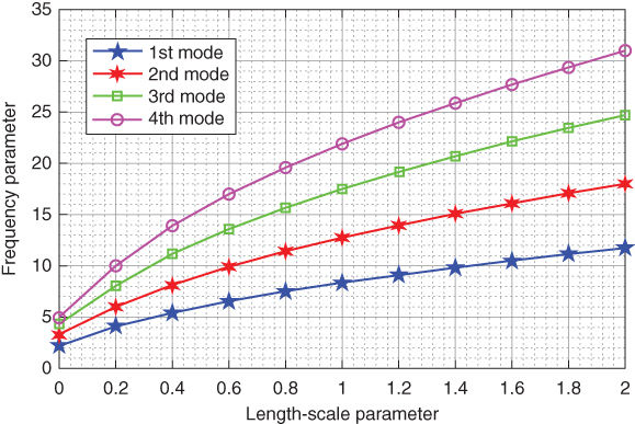
Figure 12.8 Frequency parameter vs. length‐scale parameter for CC boundary condition.
12.6 Conclusion
This chapter deals with the study of free vibration of Euler–Bernoulli nanobeam under the framework of the strain gradient model. DTM is applied for the first time to investigate the dynamic behavior of SS and CC boundary conditions. Frequency parameters of strain gradient nanobeam are validated with previously published results of research article showing robust agreement. Also, the convergence of the present results is explored, showing that CC nanobeam requires more points than that of SS boundary condition. Further, the effects of small‐scale parameters and length‐scale parameters on frequency parameters are reported through graphical and tabular results. The frequency parameters decrease with the increase of small‐scale parameters, whereas the trend of frequency parameters is opposite in the case of length‐scale parameter.
Acknowledgment
The first author is very much thankful to the Defence Research & Development Organization (DRDO), Ministry of Defence, New Delhi, India (Sanction Code: DG/TM/ERIPR/GIA/17‐18/0129/020), and the second author is also thankful to the Department of Science and Technology, Government of India, for providing INSPIRE fellowship (IF170207) to undertake the present research work.
References
- 1 Aifantis, E.C. (1992). On the role of gradients in the localization of deformation and fracture. International Journal of Engineering Science 30: 1279–1299.
- 2 Mindlin, R.D. and Tiersten, H.F. (1962). Effects of couple‐stresses in linear elasticity. Archive for Rational Mechanics and Analysis 11: 415–448.
- 3 Yang, F.A.C.M., Chong, A.C.M., DCC, L., and Tong, P. (2002). Couple stress based strain gradient theory for elasticity. International Journal of Solids and Structures 39: 2731–2743.
- 4 Eringen, A.C. (1972). Nonlocal polar elastic continua. International Journal of Engineering Science 10: 1–16.
- 5 Chakraverty, S. and Jena, S.K. (2018). Free vibration of single walled carbon nanotube resting on exponentially varying elastic foundation. Curved and Layered Structures 5: 260–272.
- 6 Jena, S.K. and Chakraverty, S. (2018). Free vibration analysis of Euler–Bernoulli nanobeam using differential transform method. International Journal of Computational Materials Science and Engineering 7: 1850020.
- 7 Jena, S.K. and Chakraverty, S. (2018). Free vibration analysis of variable cross‐section single layered graphene nano‐ribbons (SLGNRs) using differential quadrature method. Frontiers in Built Environment 4: 63.
- 8 Jena, S.K. and Chakraverty, S. (2018). Free vibration analysis of single walled carbon nanotube with exponentially varying stiffness. Curved and Layered Structures 5: 201–212.
- 9 Jena, R.M. and Chakraverty, S. (2018). Residual power series method for solving time‐fractional model of vibration equation of large membranes. Journal of Applied and Computational Mechanics 5: 603–615.
- 10 Jena, S.K. and Chakraverty, S. (2019). Differential quadrature and differential transformation methods in buckling analysis of nanobeams. Curved and Layered Structures 6: 68–76.
- 11 Jena, S.K., Chakraverty, S., Jena, R.M., and Tornabene, F. (2019). A novel fractional nonlocal model and its application in buckling analysis of Euler–Bernoulli nanobeam. Materials Research Express 6: 1–17.
- 12 Jena, S.K., Chakraverty, S., and Tornabene, F. (2019). Vibration characteristics of nanobeam with exponentially varying flexural rigidity resting on linearly varying elastic foundation using differential quadrature method. Materials Research Express 6: 1–13.
- 13 Jena, S.K., Chakraverty, S., and Tornabene, F. (2019). Dynamical behavior of nanobeam embedded in constant, linear, parabolic and sinusoidal types of winkler elastic foundation using first‐order nonlocal strain gradient model. Materials Research Express 6 (8): 0850f2. 1–23.
- 14 Jena, R.M., Chakraverty, S., and Jena, S.K. (2019). Dynamic response analysis of fractionally damped beams subjected to external loads using homotopy analysis method. Journal of Applied and Computational Mechanics 5: 355–366.
- 15 Akgöz, B. and Civalek, Ö. (2012). Analysis of micro‐sized beams for various boundary conditions based on the strain gradient elasticity theory. Archive of Applied Mechanics 82: 423–443.
- 16 Akgöz, B. and Civalek, Ö. (2013). A size‐dependent shear deformation beam model based on the strain gradient elasticity theory. International Journal of Engineering Science 70: 1–14.
- 17 Ansari, R., Gholami, R., and Sahmani, S. (2011). Free vibration analysis of size‐dependent functionally graded microbeams based on the strain gradient Timoshenko beam theory. Composite Structures 94: 221–228.
- 18 Ansari, R., Gholami, R., Shojaei, M.F. et al. (2013). Size‐dependent bending, buckling and free vibration of functionally graded Timoshenko microbeams based on the most general strain gradient theory. Composite Structures 100: 385–397.
- 19 Kahrobaiyan, M.H., Rahaeifard, M., Tajalli, S.A., and Ahmadian, M.T. (2012). A strain gradient functionally graded Euler–Bernoulli beam formulation. International Journal of Engineering Science 52: 65–76.
- 20 Khaniki, H.B. and Hosseini‐Hashemi, S. (2017). Buckling analysis of tapered nanobeams using nonlocal strain gradient theory and a generalized differential quadrature method. Materials Research Express 4: 065003.
- 21 Li, L., Li, X., and Hu, Y. (2016). Free vibration analysis of nonlocal strain gradient beams made of functionally graded material. International Journal of Engineering Science 102: 77–92.
- 22 Li, L., Hu, Y., and Li, X. (2016). Longitudinal vibration of size‐dependent rods via nonlocal strain gradient theory. International Journal of Mechanical Sciences 115: 135–144.
- 23 Lim, C.W., Zhang, G., and Reddy, J.N. (2015). A higher‐order nonlocal elasticity and strain gradient theory and its applications in wave propagation. Journal of the Mechanics and Physics of Solids 78: 298–313.
- 24 Li, L. and Hu, Y. (2015). Buckling analysis of size‐dependent nonlinear beams based on a nonlocal strain gradient theory. International Journal of Engineering Science 97: 84–94.
- 25 Li, X., Li, L., Hu, Y. et al. (2017). Bending, buckling and vibration of axially functionally graded beams based on nonlocal strain gradient theory. Composite Structures 165: 250–265.
- 26 Lu, L., Guo, X., and Zhao, J. (2017). Size‐dependent vibration analysis of nanobeams based on the nonlocal strain gradient theory. International Journal of Engineering Science 116: 12–24.
- 27 Şimşek, M. (2016). Nonlinear free vibration of a functionally graded nanobeam using nonlocal strain gradient theory and a novel Hamiltonian approach. International Journal of Engineering Science 105: 12–27.
- 28 Zhou, J.K. (1986). Differential Transformation and its Application for Electrical Circuits, 196–102. Huazhong University Press.
- 29 Chen, C.K. and Ho, S.H. (1999). Solving partial differential equations by two‐dimensional differential transform method. Applied Mathematics and Computation 106: 171–179.
- 30 Ayaz, F. (2003). On the two‐dimensional differential transform method. Applied Mathematics and Computation 143: 361–374.
- 31 Ayaz, F. (2004). Solutions of the system of differential equations by differential transform method. Applied Mathematics and Computation 147: 547–567.
- 32 Ozdemir, O. and Kaya, M.O. (2006). Flapwise bending vibration analysis of a rotating tapered cantilever Bernoulli–Euler beam by differential transform method. Journal of Sound and Vibration 289: 413–420.
- 33 Ozdemir, O. and Kaya, M.O. (2006). Flapwise bending vibration analysis of double tapered rotating Euler–Bernoulli beam by using the differential transform method. Meccanica 41: 661–670.
- 34 Balkaya, M., Kaya, M.O., and Sağlamer, A. (2009). Analysis of the vibration of an elastic beam supported on elastic soil using the differential transform method. Archive of Applied Mechanics 79: 135–146.
- 35 Ozgumus, O.O. and Kaya, M.O. (2010). Vibration analysis of a rotating tapered Timoshenko beam using DTM. Meccanica 45: 33–42.
- 36 Zarepour, M., Hosseini, S.A., and Ghadiri, M. (2017). Free vibration investigation of nanomass sensor using differential transformation method. Journal of Applied Physics A 181: 1–10.
- 37 Nourifar, M., Keyhani, A., and Aftabi Sani, A. (2018). Free vibration analysis of rotating Euler–Bernoulli beam with exponentially varying cross‐section by differential transform method. International Journal of Structural Stability and Dynamics 18: 1850024.
- 38 Wang, C.M., Zhang, Y.Y., and He, X.Q. (2007). Vibration of nonlocal Timoshenko beams. Nanotechnology 18: 105401.