
Glass molding process for microstructures
T. Zhou1 and J. Yan2, 1Beijing Institute of Technology, Beijing, P.R. China, 2Keio University, Yokohama, Japan
Abstract
Microstructures are increasingly applied in optical systems, precision measurement, arms navigation, biomedical fields, and so on. Microstructures include microgrooves, micropatterns, microprisms, and microlenses. This chapter provides an overview of the application of microstructures and glass molding processes. It highlights commonly used materials for glass molding processes; the materials to fabricate the mold are also introduced. The latest examples of glass molding simulations are discussed, including viscoelastic constitutive modeling, the microstructure molding process, and a simulation coupling heat transfer and viscous deformation. Molding quality control and molding defects in a glass molding process are also introduced in this chapter.
Keywords
Microgroove; microstructure; microlenses; glass molding; viscoelastic modeling; FEM simulation
8.1 Application of microstructures
8.1.1 Optical imaging in an optical system
8.1.1.1 Refraction
Refraction is the change in direction of propagation of a wave due to a change in its transmission medium, and optical components with microstructures have many applications based on the refraction function in the optical system.
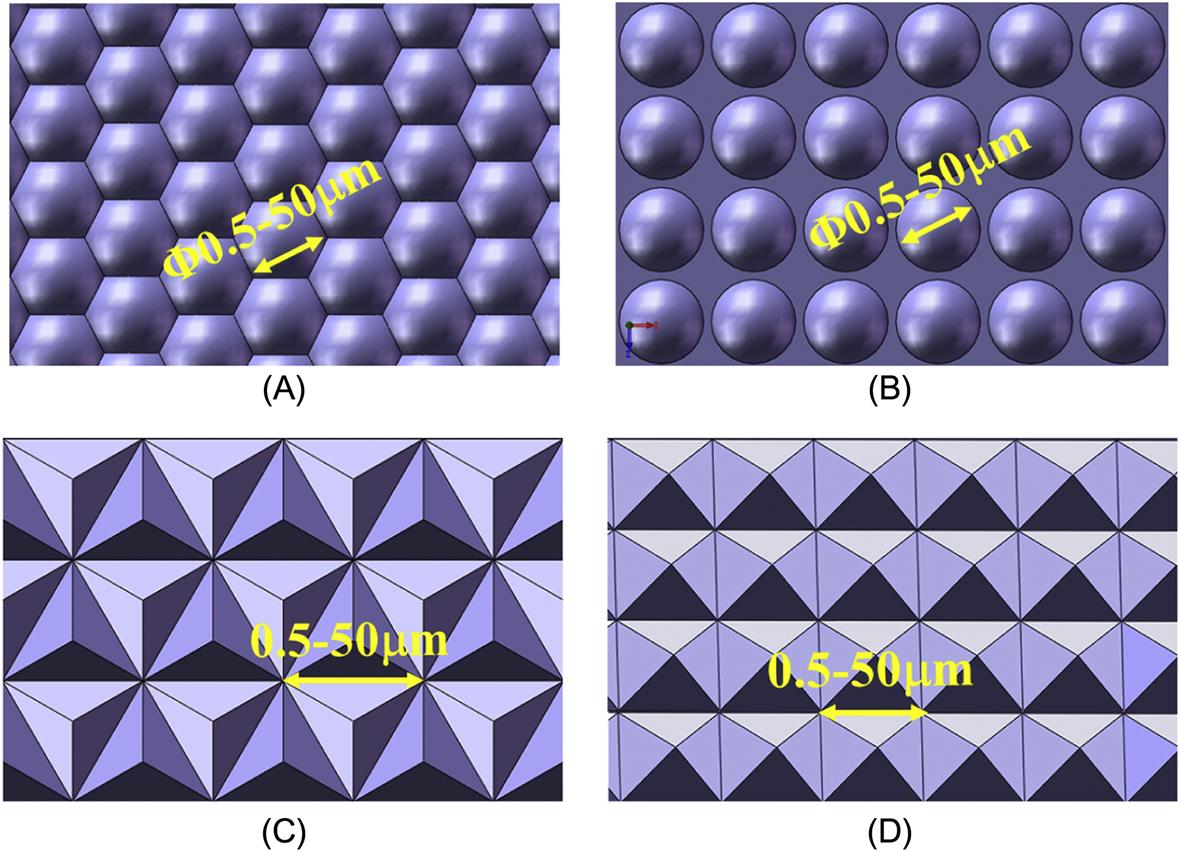
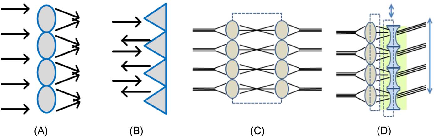
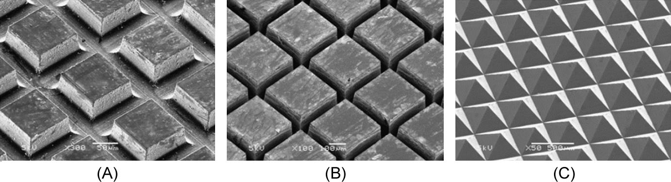
Microstructure arrays are configurations of a number of lenses or prisms in a micro-nanoscale and can provide a variety of optical functions due to their special geometrical features. The basic types of microstructure arrays are displayed in Fig. 8.1 according to the element shape. Microstructure arrays with large element size, for instance, 0.5~50 μm, mainly achieve optical performance by their refraction and reflection properties. They can raise light energy utilization ratio and realize miniaturization of optical systems through multiple imaging. Moreover, a combination of several types of microstructure arrays is able to contribute to beam guidance control, smart scan and other complex functions (shown in Fig. 8.2). Due to these functions, microstructure arrays are widely used in LCD, mobile phones, palm pilots, TVs and other electrical products.
An example of microstructures based on the refraction principle is a wave-front sensor, which is composed of microlens array and CCD (charge-coupled device) array. A Shack-Hartmann wave-front sensor can be used to characterize the performance of an optical system. In addition, they are increasingly being used to control the adaptive optical elements by real-time monitoring of wave-fronts in order to achieve the goal that eliminates the wave-front distortion before the imaging.
8.1.1.2 Diffraction
Diffraction, which is defined as the bending of light around the corners of an obstacle or aperture into the region of geometrical shadow of the obstacle, is another significant property of microstructures.
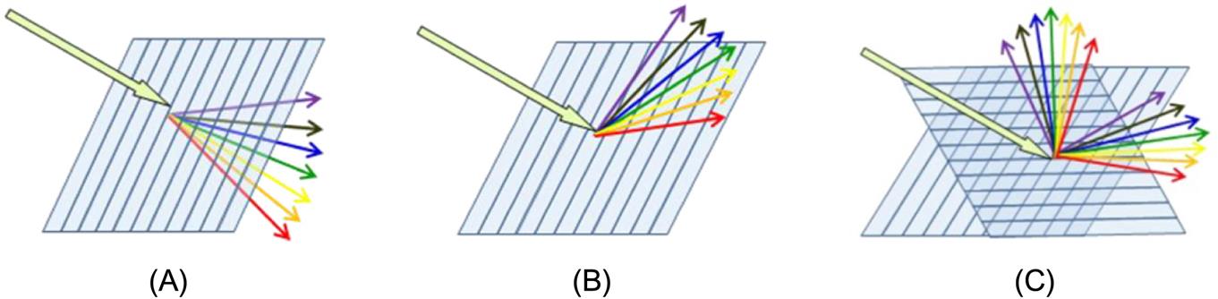
Microstructure arrays with small element size, for instance, 0.5~5 μm, mainly achieve optical performance by their interference and diffraction reflection properties. They can produce entirely different phenomena compared with macro lenses when light goes through microstructure arrays. As shown in Fig. 8.3, microstructure arrays are equipped with properties of one-dimensional diffraction and two-dimensional diffraction. They are probably able to accomplish antireflection and other goals such as polarization beam splitting, optical waveguide coupling, light beam transformation and integration if we focus on the complicated design of cycle structures and the shape of microstructure arrays.
The most common use of optical components with microstructures based on diffraction principle is diffraction grating, which is a component of optical devices consisting of a surface ruled with close, equidistant and parallel lines for the purpose of resolving light into spectra. As a typical application of diffraction grating, optical spectrometers are widely applied in the field of process control, plasma diagnostics, spectroscopic analysis of gases and liquids (Gruger, Wolter, Schuster, Schenk, & Lakner, 2003). The working principle of a spectrometer is shown in Fig. 8.4. The electrons enter into the magnet gap from the O point placed at the accelerator isocenter. An image plate shielded by lead is used to detect the electrons that are deflected between the two magnets.

The diffraction grating can also be used in the imaging system, fiber grating, and encoder. However, one of the most important usages of diffraction grating is the sensor that is used in machine tools and measurement equipment.
8.1.2 Positioning sensor in machine tools and measurement equipment
8.1.2.1 Linear grating
There are hundreds of types of positioning sensors in machine tools, and the simplest one is the grating ruler, which is used as the checkout gear in the numerical control machine tool.
In the installation process for a grating ruler, the line on the indicator grating will generate a small angle with the line on the ruler grating, and these lines on two gratings cross each other. The lines overlap and form black fringes near the intersection and bright fringes in other places when light goes through the grating. These fringes are called moiré fringes (shown in Fig. 8.5).
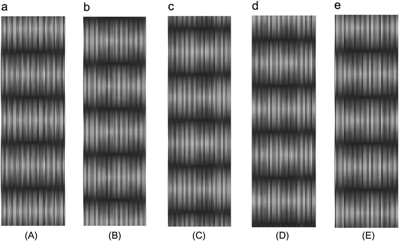
The moiré fringes change between the bright and the dark with the movement of grating. After signal processing, circuit amplification, shaping and differential, the system will output the pulse. Each output of a pulse is represented by the distance of a grid. By counting the pulses, the moving distance of the working table can be obtained.
8.1.2.2 Face grating
In optics, face grating is an optical component with a periodic structure on the surface, which splits and diffracts light into several beams traveling in different directions. With the development of ultraprecision numerical control manufacturing technology, the machining precision of ultraprecision machine tools has reached the submicron scale shape precision and nanoscale surface roughness, which directly dependends on strict control of the drive and ultraprecision testing technology.
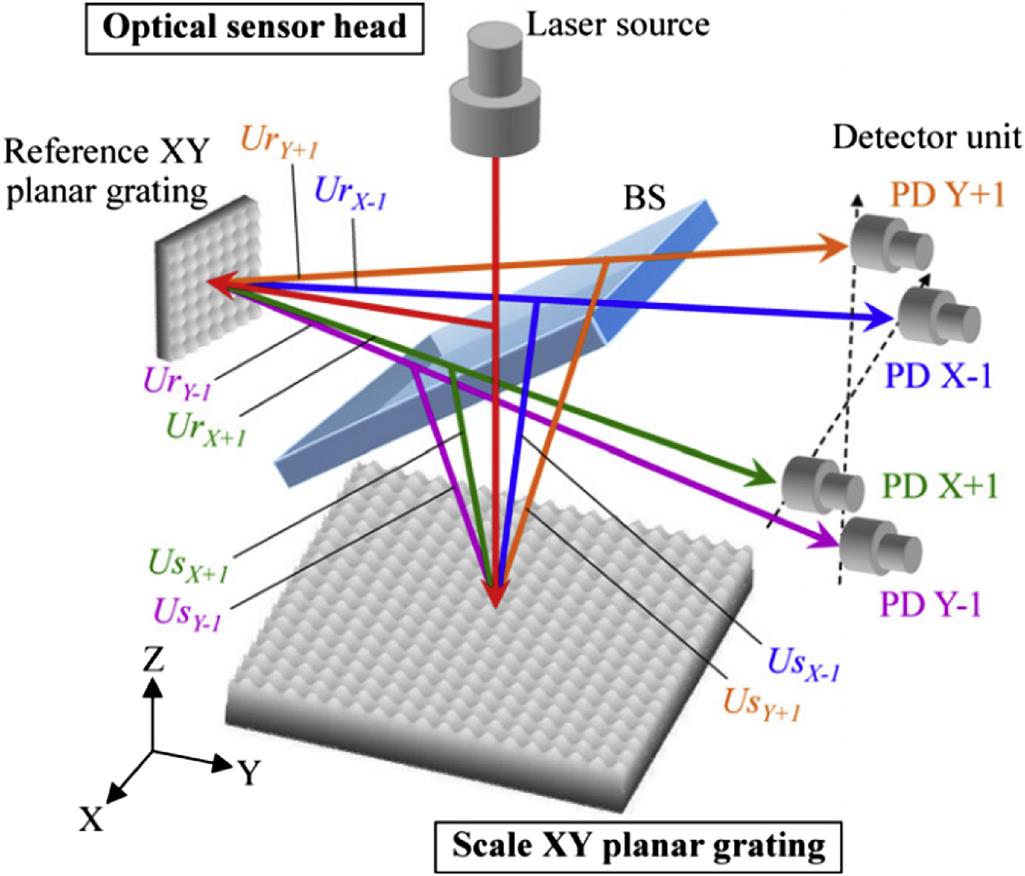
Fig. 8.6 shows the fundamental structure of the three-axis surface encoder, which is composed of an optical sensor head and a scale XY planar grating. The scale XY planar grating has periodic grating structures with a period of ![]() in the X- and Y-axes. The components of the optical sensor head are a laser source, a nonpolarizing beam splitter (BS), a detector unit and a reference XY planar grating. A laser beam from the optical sensor head is projected onto the moving scale grating. The X-directional positive and negative first-order diffracted beams from the scale grating interfere with each other to generate interference signals, from which the X-directional displacement can be obtained. Similarly, the Y-directional displacement can be obtained from the interference between the Y-directional positive and negative first-order diffracted beams from the scale grating. The XY planar encoder has been successfully used for two-axis XY position measurements of CNC machine tools and photolithography scanners.
in the X- and Y-axes. The components of the optical sensor head are a laser source, a nonpolarizing beam splitter (BS), a detector unit and a reference XY planar grating. A laser beam from the optical sensor head is projected onto the moving scale grating. The X-directional positive and negative first-order diffracted beams from the scale grating interfere with each other to generate interference signals, from which the X-directional displacement can be obtained. Similarly, the Y-directional displacement can be obtained from the interference between the Y-directional positive and negative first-order diffracted beams from the scale grating. The XY planar encoder has been successfully used for two-axis XY position measurements of CNC machine tools and photolithography scanners.
8.1.3 Micro fluid control in a biomedical field
The microstructures are widely employed not only in optical imaging and mechanical engineering, but also in the biomedical field. For instance, they can be used in the measurement system of the deformability of red blood cells (RBC). The deformability of RBC is the ability of getting through the narrow vascular channels by their deformation when the RBC are in the flow process, which is one of the most significant blood rheology indexes. Therefore, the study of RBC deformability has played an important role in preventing and curing some diseases because of RBC morphological features.
A cell deformability analysis system, based on MEMS and microfluidic technology, is useful for simulating capillaries (shown in Fig. 8.7), improving flow path and driving mode. It also combines with the enhancement of a high-speed image acquisition system (shown in Fig. 8.8) and static and dynamic image processing when using a microchannel array.

Compared with normal rheological detection technology, this method is advanced in many aspects, such as multiinformation, flexible, controllable structure, easy to handle and low cost. In addition, this approach is objective and can provide a valuable reference for the auxiliary diagnosis of relative diseases, as well as other applications in the fields of biomedicine and biomedical engineering.
8.2 Fundamental of glass molding technique
8.2.1 Introduction
Three-dimensional microsurface structures such as microgrooves, micropyramids, microprisms and microlenses are demanded more and more in recent optical, optoelectronic, mechanical and biomedical industries. Components with microsurface structures yield new functions for light operation, thereby improving significantly the imaging quality of optical systems. Microgrooves can also be used as fluid channels in biomedical and biochemical applications. Therefore, high-precision and high efficiency fabrication of microgrooves on flat or curved surfaces are receiving focused interests (Zhou, Yan, Masuda, Oowada, & Kuriyagawa, 2011).
Commercially, glass and plastic are two major substrate materials for microstructured components. Glass has predominant advantages over plastic in aspects of hardness, refractive index, light permeability, stability to environmental changes in terms of temperature and humidity, etc. A few microstructures on glass can be fabricated by material removal processes, such as sand blasting, photolithography, wet/dry etching and focused ion beam (FIB), and so on. These processes are effective for manufacturing microstructures with rectangular cross-sections (U-grooves), but it is difficult to fabricate microgrooves with sharp-angled cross-sections (V-grooves). Microcutting of glass using microendmills has also been reported, but the production efficiency is limited and the production cost is considerably high for mass production. As an alternative approach, glass molding process (GMP) is able to produce glass optical elements by replicating the shape of the mold to heated glass preforms without further machining process. Fig. 8.9 shows the glass molding process technology of the microstructure array.

From the viewpoint of fabrication cost and process time, the GMP is undoubtedly a better approach to produce precision optical elements, such as aspherical lenses, Fresnel lenses, diffractive optical elements (DOEs), microprism arrays and microlens arrays. In recent years, glass molding for microstructure, alternatively termed hot embossing or thermal imprinting, has also been reported.
The production of precision glass lenses with microgrooves by hot compression molding is a promising manufacturing method in terms of saving production costs and environment compatibility. It has shown that the molding process can produce lenses with form accuracy, surface finish and an optical performance that is comparable to lenses manufactured by conventional material removal techniques. Fig. 8.10 shows the process flow of microgroove forming. According to the thermal cycle, the process can be divided into four stages: heating, pressing, annealing, and cooling. Firstly, a glass preform is placed on the lower mold and inert gas, such as nitrogen (N2), is flowed to purge the air in the machine chamber; then the molds and glass preform are heated to the molding temperature by a heat source, such as infrared lamps (Fig. 8.10A). Secondly, the glass preform is pressed by closing the two mold halves (Fig. 8.10B). Thirdly, while a small pressing load is maintained, the formed lens is slowly cooled down to release the internal stress, namely, annealing (Fig. 8.10C). Finally, the glass lens is cooled rapidly to ambient temperature and released from the molds (Fig. 8.10D). Through these four stages, the shapes of the mold cores are precisely replicated to the glass lens.

However, in the process of microgroove forming, there are several technical challenges associated with the molding process which have prevented it from being applicable in industry for high-volume lens production. These challenges include thermal shrinkage of the lens on cooling, optical surface finish and precise mold shape, mold life and the selection of process parameters.
8.2.2 Materials suited for optical microstructures molding
8.2.2.1 Polymethyl methacrylate
Polymethyl methacrylate (PMMA) is a transparent, tough and rigid plastic. Some detail characteristics are illustrated in Table 8.1. Its properties remain stable when exposed to ultraviolet radiation and terrible conditions. Therefore, it is an ideal substitute for glass. PMMA is widely employed in domed skylights, swimming pool enclosures, aircraft canopies, instrument panels and luminous ceilings. For these applications, the plastic is drawn into sheets that are machined or thermoformed, and it is also injection-molded into automobile lenses and lighting-fixture covers. PMMA is frequently made into optical fibers for telecommunication or endoscopy because of its unusual property of keeping a beam of light reflected within its surfaces.
Table 8.1
Basic properties of PMMA (Smith & Hashemi, 2011)
| Chemical formula | (C5O2H8)n |
| Molar mass | Varies |
| Density | 1.18 g/cm3 |
| Melting point | 160°C (320°F; 433K) |
| Refractive index (nD) | 1.4905 (at 589.3 nm) |
Due to the outstanding performance in the optical system, PMMA can also be used for microstructure fabrication. In injection molding process, the PMMA solutions with the concentration of 9.1% are prepared in the solvents of benzene and methyl methacrylate (MMA) separately. The solution is spin-coated on the glass substrate at the speed of 1000 r/min for 30 s, and then gradually heated up to 100°C. The patterned surface of a polydimethylsiloxane (PDMA) stamp is contacted closely with PMMA film, and kept at 120°C for about 4 h under a certain pressure. Having removed off the PDMS stamp gently, the cylindrical micropattern on the PMMA film, the same as that on the template, is obtained. The cylindrical microlens array of PMMA film on the glass substrate is kept at the temperature beyond its softened temperature for a suitable time period until every microcylinder is completely shrunk into a hemispherical lens.
8.2.2.2 Low-melting optical glass
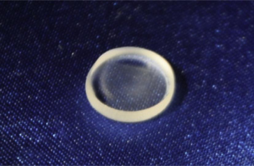
The low-melting optical glass has a low melting point, which is suitable for molding. This kind of optical glass is made by mixing high-purity silicon oxide, boron, sodium, potassium, zinc, lead, magnesium, calcium, barium and other oxide in a specific recipe. The glass usually melts in a platinum crucible with high temperature at first. Then it is stirred well and gets away from the bubble in ultrasound. Finally internal stress is removed after a long, slow cooling and annealing process. At this point the manufacture of low-melting optical glass is completed, and the molding process can be carried out. The molded glass aspheric lens is shown in Fig. 8.11.
The glass with high softening point temperature needs a high forming point temperature. In high-temperature conditions the glass may involve with physical or chemical reaction with the mold which shortens the service life of the mold. From the viewpoint of prolonging the service life of the mold, we should develop the glass material which is suitable for low temperature (under 600°C).
The low-melting optical glass is one of the most important materials of the GMP. It can be used not only in the manufacture of the lens with normal size, but also to mold the microlens arrays. As a result, the products can get an excellent service performance due to its excellent optical and physical properties.
8.2.2.3 Infrared Materials
The Infrared Materials is a general term of several kinds of materials and the most common use is the chalcogenide glass, which contains one or more chalcogenide elements (not counting oxygen). Glass-forming abilities decrease with increasing molar weight of constituent elements, i.e., S>Se>Te.
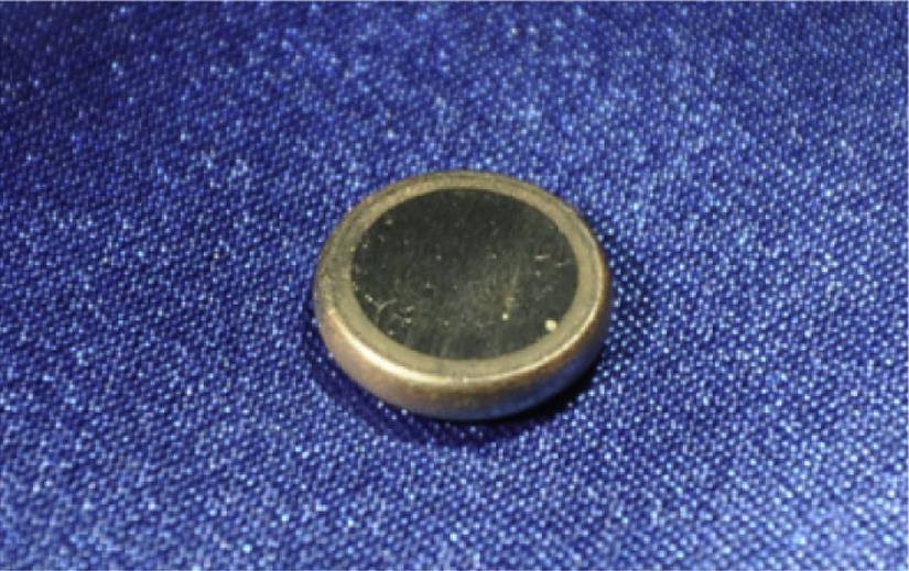
Chalcogenide glass, as shown in Fig. 8.12, is widely used in various aspects of industrial systems. The semiconducting properties of chalcogenide glasses were revealed in 1955 by B.T. Kolomiets and N.A. Gorunova from Loffe Institute, USSR (Kolomiets, 1964a, 1964b). This discovery initiates numerous researches and applications of this new semiconducting material. Modern chalcogenide compounds such as AgInSbTe and GeSbTe, are in widespread application in rewritable optical disks and phase-change memory devices. However, the most important application is in the infrared field including infrared detectors, moldable infrared lenses and infrared optical fibers, with the main advantage that these materials transmit across a wide range of the infrared electromagnetic spectrum. The physical properties of chalcogenide glasses (high refractive index, low phonon energy and high nonlinearity) also make them ideal for incorporating into lasers, planar optics, photonic integrated circuits and other active devices especially if rare earth ions are added.
Chalcogenide glasses is also moldable, which means complex shapes can be developed without using traditional expensive processes such as single point diamond turning (SPDT) or polishing. A molding method significantly lowers cost and improves production, so nowadays many chalcogenide glasses lenses are made by the GMP.
8.2.3 Mold material
8.2.3.1 Commonly used mold material
In the molding/embossing/imprinting process, mold fabrication is an important issue. Silicon or nickel molds, usually employed for polymer forming, cannot be used for glass forming because of their poor heat resistance and difficulty of removal arising from cohesion between the mold and glass. Super-hard materials, such as silicon carbide (SiC) and tungsten carbide (WC), are preferable mold materials for pressing continuous surfaces like aspherical lenses.
Silicon carbide (SiC), exceedingly hard, is synthetically produced by crystalline compound of silicon and carbon. Silicon carbide was the hardest synthetic material known until the invention of boron carbide in 1929. It has a Mohs hardness rating of 9, approaching that of diamond. In addition to hardness, silicon carbide crystals have fracture characteristics that make them extremely useful for grinding wheels, abrasive paper and cloth products. Its high thermal conductivity, together with its high-temperature strength, low thermal expansion, and resistance to chemical reaction, make it valuable in the manufacture of high-temperature glass molds and other refractories.
Tungsten carbide (WC) is a chemical compound containing equal parts of tungsten and carbon atoms. It can be pressed and formed into shapes for use in industrial machinery, cutting tools, abrasives, armor-piercing rounds, other tools and instruments, and jewellery. Tungsten carbide is approximately twice stiffer than steel, with a Young’s modulus of approximately 530~700 GPa (Groover, 2007; Sloely, 2001), and is double the density of steel, which is nearly midway between that of gold. It is comparable with corundum (α-Al2O3) in hardness and can only be polished and finished with abrasives of superior hardness such as cubic boron nitride and diamond powder, wheels and compounds. The other properties of the tungsten carbide are shown in the Table 8.2.
Table 8.2
Properties of Tungsten carbide (Cardarelli, 2008)
| Chemical formula | WC |
| Molar mass | 195.85 g/mol |
| Appearance | Gray-black lustrous solid |
| Density | 15.6 g/cm3 |
| Melting point | 2785~2830°C (5045~5126°F; 3058~3103K) |
| Boiling point | 6000°C (10,830°F; 6270K) at 760 mmHg |
| Solubility in water | Insoluble |
But the chemical reaction, stress and repeated heat treatment on the surface of glass will affect the life of the mold core. The glass adhering to the mold surface, the oxidation, and the wear of the mold greatly reduce the service life of mold. The mold and glass materials at high temperature will produce quite an intense chemical reaction, ion exchange reaction and heat reaction, thereby leading mutual diffusion or generating new compounds in the interface. Therefore, it is highly necessary to deal with the surface of the mold. Ni-P coating (shown in Fig. 8.13) can effectively solve the problem by retarding the surface reaction so as to reduce mechanical damage during hot pressing.

These materials have not been commonly used for molding microstructures, since they are very difficult to generate microstructures. In embossing/imprinting research, glassy carbon (GC) molds fabricated by FIB or dicing are used at present.
Glass-like carbon, often called GC or vitreous carbon, is a nongraphitizing carbon that combines glassy and ceramic properties. The most important properties are high-temperature resistance, high hardness (7 Mohs), low density, low electrical resistance, low friction, low thermal resistance, extreme resistance to chemical attack, and impermeability to gases and liquids. GC is widely used as an electrode material in electrochemistry, as well as for high-temperature mold (shown in Fig. 8.14). As a component of some prosthetic devices, it can be fabricated as different shapes, sizes and sections.

The reason why GC is used to make the mold of the GMP is that GC is suitable for a high temperature of 1400°C, comparable to the transition temperature of quartz glass. Another reason is that cohesion between GC and glasses is generally poor, and we can release the structure easily after embossing (Takahashi, Murakoshi, Maeda, & Hasegawa, 2007).
Normally the methods of the MEMS, like the FIB technique, are used to generate nanometer-level microstructures on a small-area GC mold, and the dicing technique is used for fabricating bigger microstructures on a large-area mold.
8.2.3.2 Mold machining method
There are various methods of MEMS to fabricate the mold of the microstructure of the glass, such as FIBs, femtosecond lasers and KrF eximer lasers (Youn, Takahashi, Goto, & Maeda, 2006). At present, the micro/nanomachining of GC is usually employed by a FIB to fabricate a mold for glass embossing (see Fig. 8.15). FIB machining characteristics are investigated with respect to accuracy, resolution, roughness and aspect ratio. Glass-embossed structures are successfully fabricated by hot molding using a GC mold (Takahashi, Sugimoto, & Maeda, 2005).

In above-mentioned text, micro/nano imprinting is developed for Pyrex glasses using a GC mold prepared by FIB machining. The disadvantage of FIB machining is the limited area of etching, the typical area of which is less than several hundred square micrometers. This is the reason that researchers tried the large area of embossing using GC mold fabricated by using a dicing machine as shown in Fig. 8.16.
Machining methods of mold consist of dicing and grinding, when the mold is used to fabricate the glass lens which is in macro size. It means this method is usually not amenable to the manufacture of the microstructure mold.
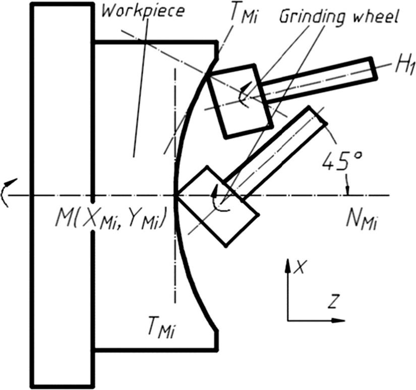
In the Cartesian coordinate system, the grinding area is the arc area of the grinding wheel side face and end face due to the high speed. In the process of ultraprecision grinding, the lens die and the grinding wheel are in point contact as shown in Fig. 8.17, which is beneficial to the control of the machining track and the subsequent compensation. Furthermore, it is easy to improve the quality of the grinding process by repairing the grinding wheel. Especially in the processing of microaspheric lens die, we can effectively avoid the interference problem by controlling the rotation of the B axis.
8.2.3.3 New mold plating material
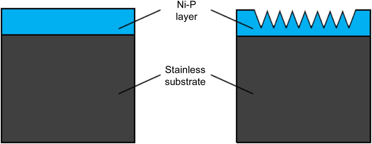
Nickel–phosphorous (Ni-P) electroless plating has been known as an important mold surface preparation technology for manufacturing plastic optical parts. Ni-P plating provides hard, wear- and corrosion-resistant surfaces at relatively high temperatures, and at the same time, maintains excellent precision micromachinability. In previous work, researchers have demonstrated that Ni-P plating can also be used for molding glass components, as shown in Fig. 8.18, such as aspherical and diffractive lenses, with a considerably long mold service life (Zhou, Liang, Wang, & Kuriyagawa, 2013).
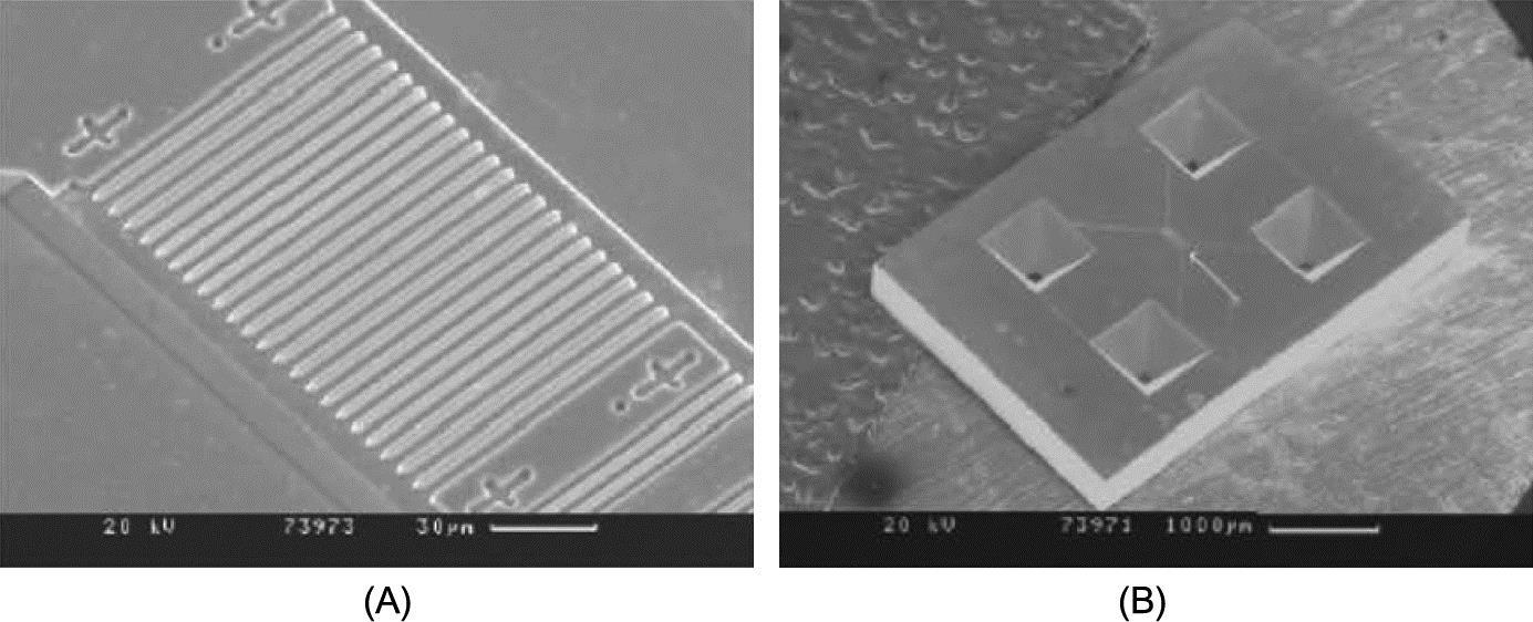
Some microcutting experiments are conducted on electroless-plated Ni-P surfaces to fabricate microstructures such as microgrooves and micropyramid arrays (shown in Fig. 8.19) (Yan, Oowada, Zhou, & Kuriyagawa, 2009).
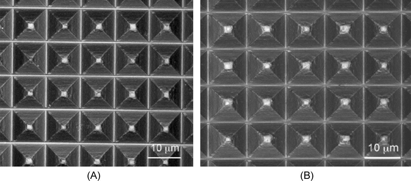
Burr formation behavior and cutting force characteristics are investigated experimentally and simulated by the finite element method (FEM) under various conditions. A simple two-step cutting process is proposed to improve the surface quality. The machined microstructure arrays are used as molds for hot-press glass molding experiments and good geometrical transferability is confirmed. The results verify that diamond-machined Ni-P microstructure molds are applicable to glass molding processes for mass production of precision microoptical components.
8.3 Modeling and simulation of microstructure molding
8.3.1 Modeling of viscoelastic constitutive
To date, there have been many attempts to simulate the behavior of viscoelastic materials. This has been aimed at facilitating analysis of the behavior of glass products, assisting with extrapolation and interpolation of experimental data and reducing the need for extensive, time-consuming creep tests. Viscoelastic behavior is the time-dependent response of a material to a strain or stress. It can be illustrated best with the help of mechanical model-combinations of springs and dashpots. A spring represents elastic or hookean behavior, and a dashpot represents viscous or Newtonian behavior. These two elements cover both parts of the notion “viscoelasticity.” In addition, a differential equation can be obtained describing the behavior of the model. The objective is to devise the model and obtain the equation that will describe the behavior of a real material (Rekhson, 1986).
Although there are no discrete molecular structures that behave like the individual elements of the models, they nevertheless do aid in the understanding and analysis of the behavior of viscoelastic materials. Several common models are shown in Fig. 8.20 (Crawford & Crawford, 1998).

8.3.1.1 The Maxwell model
The spring is the elastic component of the response and obeys the relation
(8.1)
where ![]() and
and ![]() are the stress and strain respectively and
are the stress and strain respectively and ![]() is a constant.
is a constant.
The dashpot is the viscous component of the response and in this case the stress ![]() is proportional to the rate of strain
is proportional to the rate of strain ![]() ,
,
(8.2)
where ![]() is a material constant.
is a material constant.
For equilibrium of forces, assuming a constant area. As shown in Fig. 8.20A, applied stress,
(8.3)
The total strain, ![]() is equal to the sum of the strains in the two elements. So
is equal to the sum of the strains in the two elements. So
(8.4)
From Eqs. (8.1), (8.2), and (8.4)
(8.5)
This is the governing equation of the Maxwell model. It is interesting to consider the response that this model predicts under three common-time-dependent modes of deformation.
Creep
If a constant stress ![]() is applied then Eq. (8.5) becomes
is applied then Eq. (8.5) becomes
(8.6)
which indicates a constant rate of increase of strain with time.
From Fig. 8.21 it has seen that for the Maxwell model, the strain at any time ![]() , after the application of a constant stress
, after the application of a constant stress ![]() , is given by
, is given by
(8.7)

Hence, the creep modulus, ![]() , is given by
, is given by
(8.8)
Relaxation
If the strain is held constant then Eq. (8.5) becomes
(8.9)
Solving this differential equation with the initial condition ![]() at
at ![]() then,
then,
(8.10)
(8.11)
where ![]() is referred to as the relaxation rime.
is referred to as the relaxation rime.
This indicates that the stress decays exponentially with a time constant of ![]() .
.
Recovery
When the stress is removed there is an instantaneous recovery of the elastic strain, and then, as shown by Eq. (8.5), the strain rate is zero so that there is no further recovery (see Fig. 8.21).
It can be seen therefore that although the relaxation behavior of this model is acceptable as a first approximation to the actual materials response, it is inadequate in its prediction for creep and recovery behavior.
8.3.1.2 The Kelvin model
In this model the spring and dashpot elements are connected in parallel as shown in Fig. 8.20B.
For equilibrium of forces it can be seen that the applied load is supported jointly by the spring and the dashpot, so
(8.12)
In this case the total strain is equal to the strain in each of the elements,
(8.13)
From Eqs. (8.1), (8.2), and (8.12)
(8.14)
or using Eq. (8.13)
(8.15)
This is the governing equation for the Kelvin model, and it is interesting to consider its predictions for the common-time-dependent deformations.
Creep
If a constant stress, ![]() , is applied then Eq. (8.15) becomes
, is applied then Eq. (8.15) becomes
(8.16)
and this differential equation may be solved for the total strain, ![]() , to give
, to give
(8.17)
This indicates an exponential increase in strain from zero up to the value, ![]() , that the spring would have reached if the dashpot had not been present. This is shown in Fig. 8.22. As for the Kelvin model, the creep modulus may be determined as
, that the spring would have reached if the dashpot had not been present. This is shown in Fig. 8.22. As for the Kelvin model, the creep modulus may be determined as
(8.18)
Relaxation
If the strain is held constant then Eq. (8.16) becomes
(8.19)
That is, the stress is constant and supported by the spring element so that the predicted response is that of an elastic material, no relaxation (see Fig. 8.22).
Recovery
If the stress is removed, then Eq. (8.16) becomes
(8.20)
Solving this differential equation with the initial condition ![]() at the time of stress removal, then
at the time of stress removal, then
(8.21)
This represents an exponential recovery of strain which is a reversal of the predicted creep.
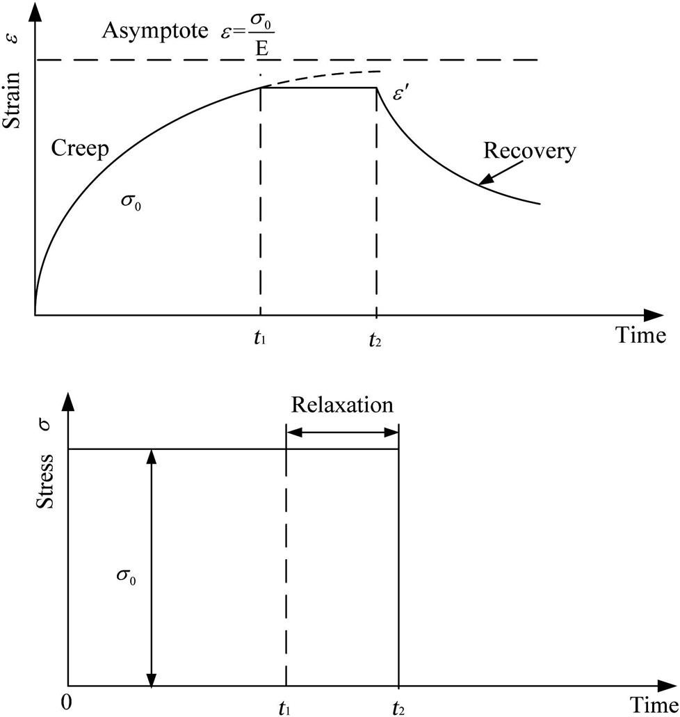
8.3.1.3 The Burger model
It can be seen that the simple Kelvin model gives an acceptable first approximation to creep and recovery behavior but does not account for relaxation. The Maxwell model can account for relaxation but was poor in relation to creep and recovery. It is clear therefore that some compromise may be achieved by combining the two models. The Burger model is shown in Fig. 8.20C, where a Maxwell and a Kelvin model are connected in a series. In this case, the stress–strain relations are again given by Eqs. (8.1) and (8.2). The geometry of deformation yields. Total strain
(8.22)
where ![]() is the strain response of the Kelvin model. From Eqs. (8.1), (8.2), and (8.22)
is the strain response of the Kelvin model. From Eqs. (8.1), (8.2), and (8.22)
(8.23)
From this the strain rate may be obtained as
(8.24)
The response of this model to creep, relaxation, and recovery situations is the sum of the effects described for the previous two models and is illustrated in Fig. 8.23. It can be seen that although the exponential responses predicted in these models are not a true representation of the complex viscoelastic response of polymeric materials, the overall picture is, for many purposes, an acceptable approximation to the actual behavior. As more and more elements are added to the model, the simulation becomes better but the mathematics become complex.

8.3.2 Simulation of microstructure molding process
With recent advances in numerical simulation capabilities and computing technology, a FEM can address some of these issues by providing deeper insight into the process and performance prediction. For a reliable simulation model, it is necessary to have accurate material representation with temperature-dependent mechanical and thermal properties. The lens molding process is usually performed at a temperature of 150–200°C above the glass transition temperature (![]() ) where the glass viscosity generally lies between 107.6 and 109.0 P. In this temperature range, also referred to as the transition temperature range, the glass can be described as a viscoelastic material exhibiting stress relaxation. Stress relaxation that influences residual stresses in a molded glass lens is therefore an important technological subject.
) where the glass viscosity generally lies between 107.6 and 109.0 P. In this temperature range, also referred to as the transition temperature range, the glass can be described as a viscoelastic material exhibiting stress relaxation. Stress relaxation that influences residual stresses in a molded glass lens is therefore an important technological subject.
The present investigation is hence undertaken to model the stress relaxation phenomenon during lens molding. It is imperative to develop a FEM-based simulation model of microgroove forming, in order to gain a fundamental understanding of the process by evaluating various parameters, which are difficult or impossible to measure during experiments. By creating a simple numerical model, we are able to predict the performance of microgroove forming process and at the same time identify the various parameters that would enable us to model the actual process.
8.3.2.1 2D modeling
Simulations of the glass molding process are conducted using a commercial FEM code MSC. Marc, which is powerful in nonlinear solution for forging and molding process of various materials. The program is capable of simulating large deformations of material flow under isothermal or nonisothermal conditions. A general Maxwell model is set up to describe the deformation during the pressing stage, as shown in Fig. 8.24. The time-dependent response is characterized by the deviatoric terms, as shown in Eq. (8.25):
(8.25)

The above integrals are evaluated for current time ![]() based on past time
based on past time ![]() .
. ![]() is not a constant value, but is represented by a Prony series as in Eq. (8.26):
is not a constant value, but is represented by a Prony series as in Eq. (8.26):
(8.26)
where ![]() is the relative moduli,
is the relative moduli, ![]() is the reduced time, used to describe the shift in time due to temperature. The shift function (
is the reduced time, used to describe the shift in time due to temperature. The shift function (![]() ) used in this model is the Tool-Narayanaswamy (TN) shift function, as shown in Eq. (8.27):
) used in this model is the Tool-Narayanaswamy (TN) shift function, as shown in Eq. (8.27):
(8.27)
where ![]() is the reference temperature.
is the reference temperature. ![]() is the activation energy, and
is the activation energy, and ![]() is the ideal gas constant.
is the ideal gas constant.
In an actual microgroove molding process, there are 500 V-grooves on the mold spacing regularly in a 5×5 mm2 area. For simplification, eight grooves are calculated in this simulation. Fig. 8.25 shows the two-dimensional simulation model of GMP for microgrooves, the upper mold, which is flat and fixed to the top, and the lower mold with microgrooves that move upward to press the softened glass. The glass object is meshed with 48,000, 3-node, triangle, and plane strain solid elements. In order to make sure the FEM simulation convergence in the contact and save the remeshing time at the sharp corner during the simulation, the sharp ridges of the grooves on the top are rounded with a radius of 1 μm on the top, while the sharp angle is held as the actual size of the valley. The molds are both modeled as rigid objects by the two curves. As the glass is pressed at the same temperature with the molds, no heat transfer is considered in this model (Zhou, Yan, Masuda, Owada, & Kuriyagawa, 2009).

Some simulation results are obtained. First, the effects of the molding temperature (![]() ) are numerically studied at 560°C, 570°C, 580°C, and 590°C, respectively. The pressing velocity (
) are numerically studied at 560°C, 570°C, 580°C, and 590°C, respectively. The pressing velocity (![]() ) is set constantly at 0.1 mm/s with a displacement of 15 μm upward. The friction coefficient (
) is set constantly at 0.1 mm/s with a displacement of 15 μm upward. The friction coefficient (![]() ) is specified to 0.1. Fig. 8.26 shows the equivalent stress distribution at the displacement of 15 μm at 570°C. The stress distributes bilaterally symmetrically on the whole glass plate, the lowest in the center groove and the highest on the left and right sides. The glass material flows from the center to the two sides and fills the center groove of the mold first; it then fills the outer grooves later. When the displacement reaches 13.74 μm, the V-groove of the mold is entirely replicated on the glass plate. The highest and the lowest stresses distribute more or less at the same area, but the peak-valley value of the stress changes fiercely.
) is specified to 0.1. Fig. 8.26 shows the equivalent stress distribution at the displacement of 15 μm at 570°C. The stress distributes bilaterally symmetrically on the whole glass plate, the lowest in the center groove and the highest on the left and right sides. The glass material flows from the center to the two sides and fills the center groove of the mold first; it then fills the outer grooves later. When the displacement reaches 13.74 μm, the V-groove of the mold is entirely replicated on the glass plate. The highest and the lowest stresses distribute more or less at the same area, but the peak-valley value of the stress changes fiercely.
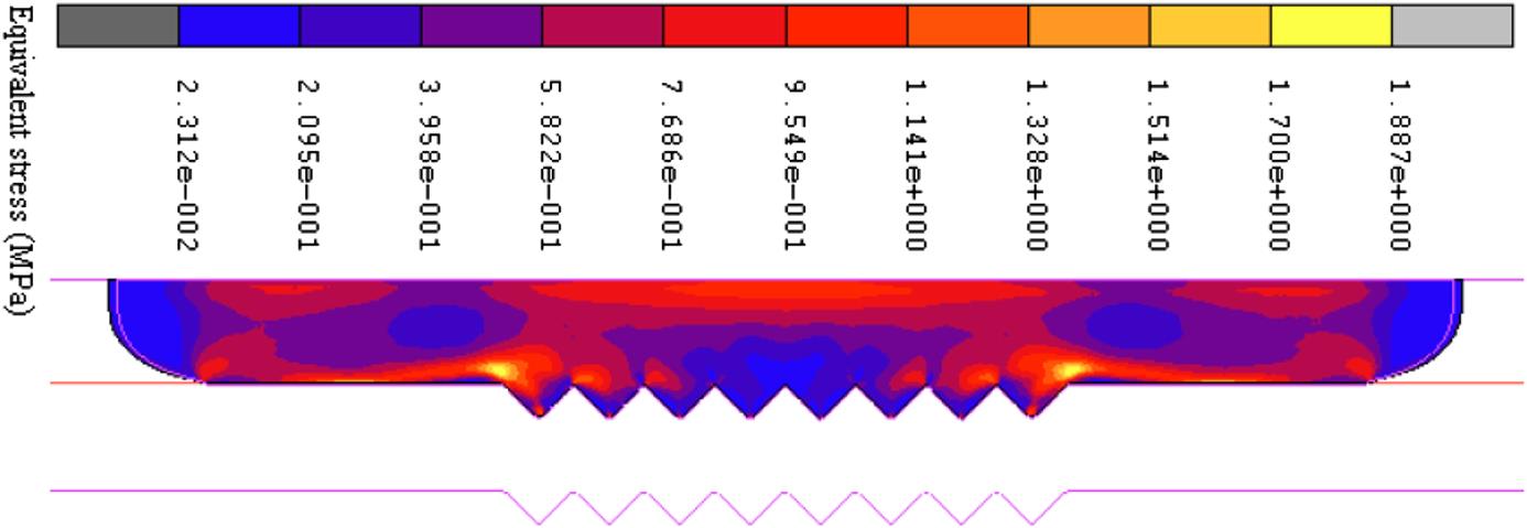
 =570°C,
  =0.1 mm/s,
  =0.1).
Second, Fig. 8.27A shows the maximum and minimum values of the equivalent stress at the temperatures from 560°C to 590°C. The lowest stress is more or less the same at different temperatures, but the highest temperature declines to 1/10 at 590°C, compared with the stress at 560°C. Also, the effects of the pressing velocity are investigated at 0.01, 0.1, and 1 mm/s, respectively. The molding temperature is fixed at 570°C. From Eq. (8.25), we know that the stress will be directly proportional to the strain rate. From the simulation results shown in Fig. 8.27B, we can find that the highest stress rises to 14.32 MPa, which is 7.6 times the highest stress at the pressing velocity of 0.1 mm/s, and 41 times the highest stress at the pressing velocity of 0.01 mm/s.
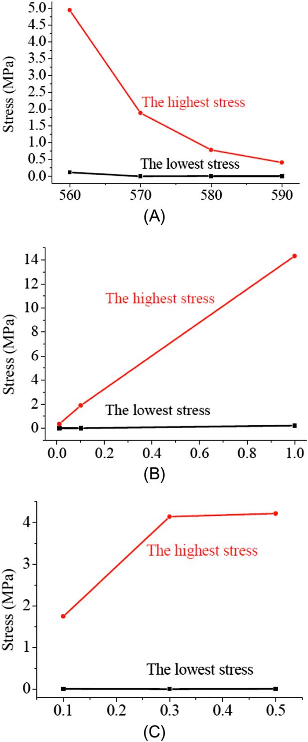
Third, as the friction coefficient on the glass-mold interface is unavailable, the coefficient is arbitrarily specified to 0.1 in the above simulation. In order to examine the effects of the friction, the GMP process is simulated by varying the friction coefficient from 0.1, 0.3, to 0.5 at the glass-mold interfaces. A true stick-up friction model is adopted. The molding temperature is 570°C. Fig. 8.27C shows the stress change at the friction coefficients of 0.1, 0.3, and 0.5. The stress at a friction coefficient of 0.3 becomes higher than that at 0.1, but does not much change when the coefficient is further increased to 0.5. Another interesting phenomenon is observed. The sharp angled V-groove can be formed at a level of less displacement when the friction becomes higher. A displacement of 13.7 μm is needed at a friction coefficient of 0.1, but only 10.8 μm at 0.3, and 10.1 μm at 0.5. The reason can be attributed to the different flow velocities of glass in the horizontal and longitudinal directions. The glass material is hard to flow in the horizontal direction at a high-friction force, and the increased pressing load results in an easy flow in the longitudinal direction. Consequently, the glass is squeezed to fill up the V-grooves with less displacement of the lower mold at a higher-friction coefficient.
A comprehensive analysis of these effects should be considered to optimize the molding condition. From the simulation results, it is shown that the molding temperature and the pressing velocity have a significant effect on the stress during the GMP process for microgrooves. Higher friction on the glass-mold interface can help to form the sharp V-grooves with a less displacement of the mold, but it will increase the stress. In fact, the friction coefficient is almost decided by the surface roughness of the mold. A lower stress can reduce the deformation of the mold and achieve a higher form accuracy. From this viewpoint, an intermediate molding temperature of 570°C, and a slow pressing velocity of 0.1 mm/s, are selected as the optimal pressing conditions in the glass molding process (GMP) experiments.
8.3.2.2 3D modeling
It is clear from the above that 2D numerical simulation is used to illustrate the details of the GMP process for microstructure, and that the molding condition has been optimized. However, the 2D simulation is not able to reveal the process of the glass material flow among microstructures forming, such as microgroove and micropyramid, because the cross-section of the V-groove is the same as that of the pyramid at the vertex. Therefore, 3D simulation is necessary in the numerical analyses of micropyramid forming and the General Maxwell model is extended to the 3D simulation. Here is an example of 3D numerical simulations that are carried out to study the forming process of microgroove array and micropyramid array (Zhou, Yan, & Kuriyagawa, 2010).
Simulations of the forming process of microgroove array and micropyramid array are conducted using a commercial FEM code MSC. Marc, which is powerful in nonlinear solutions for the forging and molding process of various materials. The 3D models of the GMP for microgrooves and micropyramids are shown in Fig. 8.28A and B, respectively.

In a real molding process, there are 500 microgrooves in a microgroove array and 500×500 micropyramids in a micropyramid array on the mold. In order to save the computing time of the FEM simulation, only 3 grooves and 3×2 pyramids are modeled in the microgroove forming and the micropyramid forming in the respective simulations. The upper flat mold, which is fixed on the top, and the lower mold with microgrooves, will move upward to press the softened glass. The glass object is meshed with 514,084-node, tetrahedral solid elements. In order to make sure of the FEM simulation convergence in the contact deformation and save the remeshing time at the sharp corner during the simulation, the sharp ridges of the microgrooves and the shape vertexes of the micropyramids are rounded with a radius of 1 μm, while the sharp angle of the valleys is held as the actual size. The molds are both modeled as rigid objects by two surfaces. As the glass is pressed at the same temperature with the molds, no heat transfer is considered in this model.
Some simulation results such as stress and strain distribution are achieved. They can be used to facilitate the comparison between microgroove forming and micropyramid forming; the 3D stress distributions and strain distributions in the glass in the GMP for both microgrooves and micropyramids are shown in the same view angle, so that the differences can be easily distinguished by comparing the corresponding parts with each other.
Fig. 8.29A and B show the stress distributions during the deformation at the displacement of 6 μm during the pressing for microgrooves and micropyramids, respectively. It demonstrates that the stress on the peaks of the microgrooves is a little higher than that on the peaks of the micropyramids, but much lower on the valleys. Therefore, a higher pressing load is needed in the GMP for microgrooves than that in the GMP for micropyramids. Furthermore, the stress concentrates on the area of the microgrooves in the microgroove forming, but the stress in the micropyramid forming scatters to the whole part of the glass.

Fig. 8.30A is the cross-section view of the molded microgrooves, which shows the strain distribution at the displacement of 6 μm during the pressing for microgrooves, and Fig. 8.30B is the cross-section view of the strain distribution for micropyramids. The strain on the peak of the microgroove is larger than that of the micropyramids. Comparing the molded microgrooves with the molded micropyramids, it shows that the horizontal deformation of the glass in the microgroove forming is larger than that in the micropyramid forming, especially on the left and right tips. Moreover, the filling ratio of the GMP for microgroove forming is a little larger than that for micropyramids.
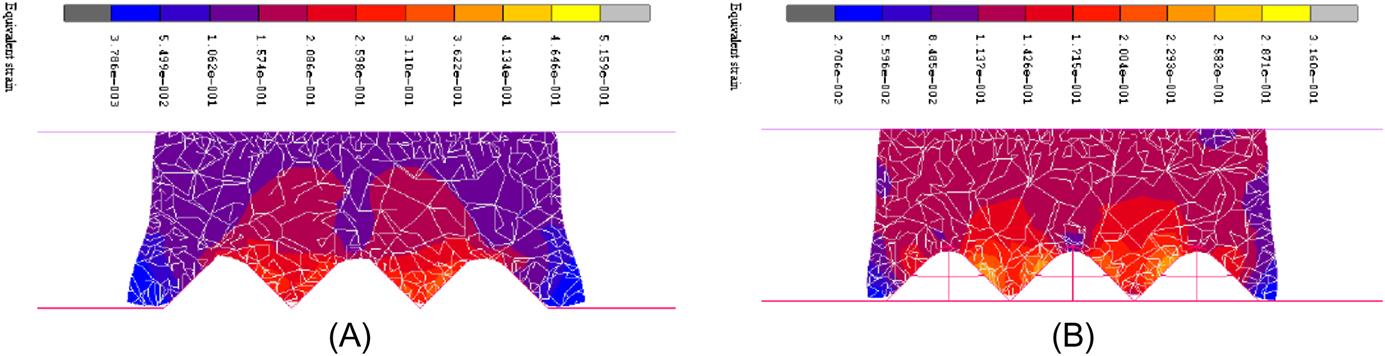
Some reasons for these differences can be generalized due to the simulation results above. First, the glass material can only flow along the two symmetric ramps of a microgroove during the pressing, but the glass material can flow along the four equal ramps of a micropyramid, just like an awl is much easier to pierce into the wood than an ax at the same pressing load. Second, the micropyramid array has almost twice the space of cavities to accommodate more glass material than the microgroove array during the pressing, so the amount of glass material flowing in the horizontal direction in the micropyramid forming process is smaller than that in the microgroove forming process. The different filling ratios of the GMP for these two kinds of microstructures have been explained by the simulation results.
8.3.3 GMP simulation coupling heat transfer and viscous deformation
In GMP, a glass preform is pressed at a temperature tens of degrees centigrade above its transition temperature to replicate the shape of the mold to the glass surface. At the molding temperature, the glass shows viscosity. Two issues are practically important in the simulation of glass molding process: one is to model heat-transfer phenomena considering the temperature dependence of specific heat and thermal conductivity of glass, and the other is to make clear the viscosity of glass near the softening point.
Since glass is transparent in infrared light, it cannot be directly heated by the infrared lamp, but instead has to be indirectly heated by the molds and the surrounding gas. Therefore, heat transfer in this case involves heat conduction, heat convection, and radiation. Also, heat expansion coefficient, heat conductivity, heat capacity and other parameters of glass are also changing with temperature. From these aspects, the heat transfer in glass molding is a very complicated issue. However, at present, precise measurement of the heat transfer in a glass lens is still difficult, although Field and Viskanta (1990) demonstrated the possibility of an experimental measurement of temperature distributions in soda-lime glass plates.
FEM has shown to be an effective approach to simulate a forming process and visualize the heat transfer in glass. For example, Wilson, Schmid, and Liu (2004) studied the heat transfer across a tool-workpiece interface by using an FEM code, DEFORMTM-2D. Viskanta and Lim (2001) proposed a physical model for internal heat transfer in glass and heat exchange across glass-mold interface in one dimension. Yi and Jain (2005) applied DEFORMTM-2D to the simulation of aspherical glass lens molding.
However, most of these studies analyzed the heating process by separately considering heat transfer and glass deformation. The numerical models they used did not take into account the time dependent and temperature-dependent changes of thermal and mechanical properties of glass, which might cause considerable simulation errors. To date, there is no available literature on the dynamic modeling of a high-temperature glass forming process by comprehensively considering the heat transfer and the thermal deformation of glass. Therefore, precise prediction of process parameters, such as heating time and pressing load, is still difficult.
In this section, a series of thermo-mechanical models coupling heat transfer and viscous deformation are established for the glass molding process, from heating, pressing, annealing to cooling, to enable FEM simulation and visualization of the process, and accurate prediction of optimal process parameters. Firstly, thermal phenomenon during the glass molding process is analyzed by considering heat transfer within glass and at the interface among glass, molds, and the surrounding gas environment. Secondly, the high-temperature viscosity of glass near the softening point is measured using an ultraprecision glass molding machine by uniaxially pressing cylindrical glass preforms between a pair of flat molds. Thirdly, the developed numerical models and the measured viscosity properties are incorporated into coupled thermo-mechanical FEM simulation of the glass pressing process based on a viscous fluid model. It shows that the developed thermal and mechanical models coupling heat transfer and viscous deformation can be used to precisely predict important process parameters of glass molding (Yan, Zhou, Masuda, & Kuriyagawa, 2009).
8.3.3.1 Theoretical models of heat transfer and viscous deformation
Thermal expansion of glass
Thermal expansion is an important issue in lens molding because it greatly influences the form accuracy of the lens. The thermal expansion of glass is strongly temperature dependent. The expansion coefficient is approximately linear at low temperature (below ![]() ), and becomes nonlinear in the high-temperature range. The thermal expansion coefficient increases significantly from
), and becomes nonlinear in the high-temperature range. The thermal expansion coefficient increases significantly from ![]() to
to ![]() , then a negative expansion (namely contraction) occurs above
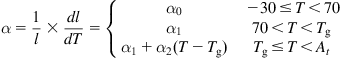
, then a negative expansion (namely contraction) occurs above ![]() . Ohlberg and Woo (1973) proposed a complicated formula to describe the change of glass expansion coefficient, but it is still hard to precisely describe the thermal expansion coefficient in a single function. For simplification, linear approximations are adopted to represent the changes of thermal expansion coefficient in different temperature ranges. To begin with, we consider the one-dimensional thermal expansion problem. The linear thermal expansion coefficient (
. Ohlberg and Woo (1973) proposed a complicated formula to describe the change of glass expansion coefficient, but it is still hard to precisely describe the thermal expansion coefficient in a single function. For simplification, linear approximations are adopted to represent the changes of thermal expansion coefficient in different temperature ranges. To begin with, we consider the one-dimensional thermal expansion problem. The linear thermal expansion coefficient (![]() ) can be given by Eq. (8.25):
) can be given by Eq. (8.25):
(8.28)
 (8.28)
where ![]() is the overall length of material in the direction being measured; T is the instantaneous temperature in
is the overall length of material in the direction being measured; T is the instantaneous temperature in ![]() ;
; ![]() is the constant thermal expansion coefficient in the working temperature range of glass;
is the constant thermal expansion coefficient in the working temperature range of glass; ![]() is the constant thermal expansion coefficient below
is the constant thermal expansion coefficient below ![]() ; and
; and ![]() is the average gradient of the increase of thermal expansion coefficient between
is the average gradient of the increase of thermal expansion coefficient between ![]() and
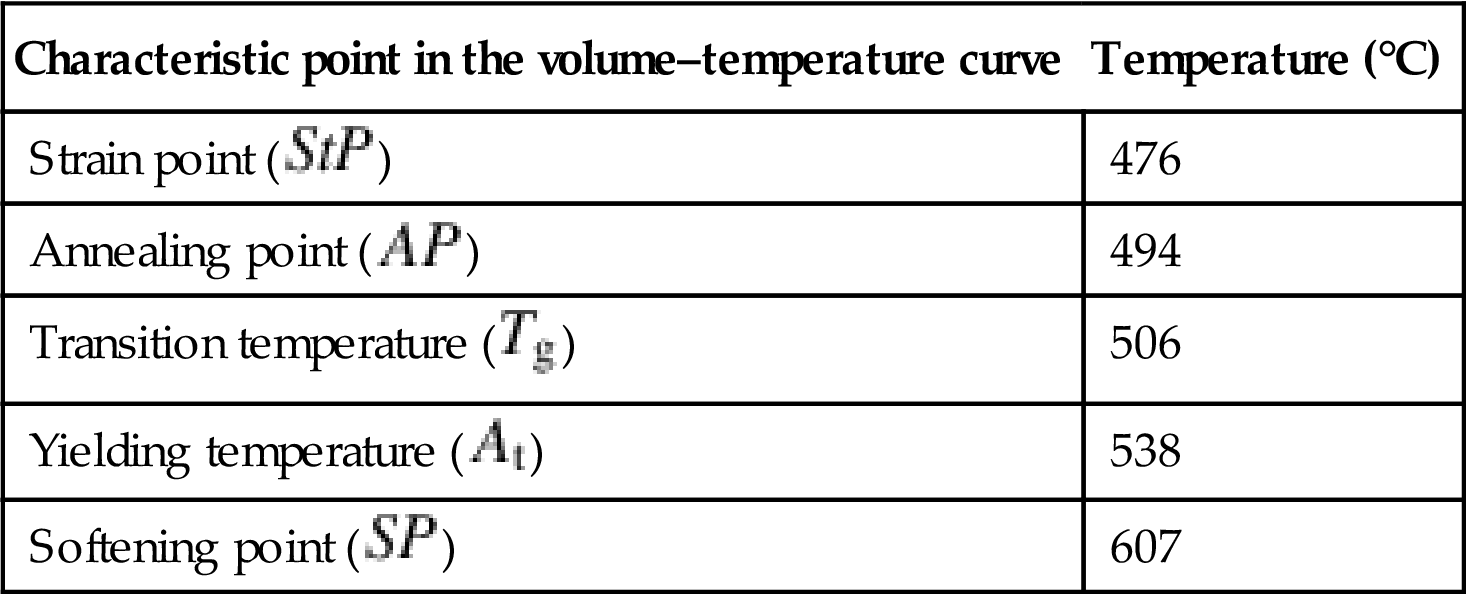
and ![]() . The glass material used in Section 3.3 is L-BAL42, the thermal characteristics of which are listed in Table 8.3. Other glasses show similar general trends in the volume–temperature curves. According to the data provided by the glass manufacturer, we obtain that
. The glass material used in Section 3.3 is L-BAL42, the thermal characteristics of which are listed in Table 8.3. Other glasses show similar general trends in the volume–temperature curves. According to the data provided by the glass manufacturer, we obtain that ![]() =7.2×10⁻⁶ L/°C,
=7.2×10⁻⁶ L/°C, ![]() =8.8×10⁻⁶ L/°C, and
=8.8×10⁻⁶ L/°C, and ![]() =3.0×10⁻⁸ L/°C2 in Eq. (8.28).
=3.0×10⁻⁸ L/°C2 in Eq. (8.28).
Table 8.3
Thermal expansion characteristics of glass L-BAL42
| Characteristic point in the volume–temperature curve | Temperature (°C) |
| Strain point ( |
476 |
| Annealing point ( |
494 |
| Transition temperature ( |
506 |
| Yielding temperature ( |
538 |
| Softening point ( |
607 |
Next, we consider volume expansion in three-dimensional glass molding. The volume thermal expansion coefficient (![]() ) is approximately three times the linear thermal expansion coefficient, thus it can be defined by Eq. (8.29). The temperature-dependent volume (
) is approximately three times the linear thermal expansion coefficient, thus it can be defined by Eq. (8.29). The temperature-dependent volume (![]() ) can then be calculated using Eq. (8.30).
) can then be calculated using Eq. (8.30).
(8.29)
(8.30)
where ![]() is the volume of glass at the reference temperature (0°C), and
is the volume of glass at the reference temperature (0°C), and ![]() is the swelling increment in volume after heating to temperature
is the swelling increment in volume after heating to temperature ![]() . In the FEM simulation of molding process, a module is activated to restore the volume change due to thermal expansion during remeshing, and the coefficient of thermal expansion is used to define the volumetric strain due to temperature changes.
. In the FEM simulation of molding process, a module is activated to restore the volume change due to thermal expansion during remeshing, and the coefficient of thermal expansion is used to define the volumetric strain due to temperature changes.
Heat transfer models
On most occasions, glass molding processes are based on the “isothermal molding” method where pressing is performed after the glass preform reaches the same temperature as the molds. However, due to the fact that the heat absorption rate of glass is distinctly different from that of the mold materials, such as tungsten carbide (WC), silicon carbide (SiC), titanium carbide (TiC), nickel–phosphorous (NiP) plated steels, and other alloys, even the glass preform and the molds are heated together by the same infrared lamp, there is a significant delay of temperature rise within the glass preform. Most of the heat transferred to the glass preform is from the lower mold and surrounding nitrogen during the soaking time. However, it is difficult to directly measure the temperature change in the glass preform even if the temperature of the molds can be easily monitored by thermocouples. Therefore, modeling of heat transfer phenomenon in glass molding is very important for working out heat balance.
Initially, we consider the heat transfer within a glass preform. The governing equation for heat conduction within an incompressible glass material is given by Eq. (8.31):
(8.31)
where ![]() is the density;
is the density; ![]() is the specific heat;
is the specific heat; ![]() is the thermal conductivity of glass; and
is the thermal conductivity of glass; and ![]() is the heating time. Most of the work on simulation of glass molding and other forming processes treated the specific capacity
is the heating time. Most of the work on simulation of glass molding and other forming processes treated the specific capacity ![]() and thermal conductivity
and thermal conductivity ![]() as constants (Choi, Ha, Kim, & Grandhi, 2004; Zhou & Li, 2005). However, in fact these two parameters are temperature-dependent, as experimentally demonstrated by early researchers (Moser & Kruger, 1968; Richet, Bottinga, & Tequi, 1984).
as constants (Choi, Ha, Kim, & Grandhi, 2004; Zhou & Li, 2005). However, in fact these two parameters are temperature-dependent, as experimentally demonstrated by early researchers (Moser & Kruger, 1968; Richet, Bottinga, & Tequi, 1984).
As glass is a compound material, the specific heat of glass is known to vary with its composition and temperature. An empirical equation, namely, Sharp–Ginther equation (Sharp & Ginther, 1951), has been proposed to express the mean specific heat (![]() ) of glass, as shown in Eq. (8.32).
) of glass, as shown in Eq. (8.32).
(8.32)
where ![]() is a constant of a glass material;
is a constant of a glass material; ![]() is the true specific heat at 0°C; and
is the true specific heat at 0°C; and ![]() is the temperature in °C.
is the temperature in °C. ![]() and
and ![]() are both decided by the glass compositions. This equation can be applied to a wide temperature range and has been widely used by later researchers.
are both decided by the glass compositions. This equation can be applied to a wide temperature range and has been widely used by later researchers.
The composition percentages of the glass samples offered by the glass manufacturer are shown in Table 8.4. An intermediate value of each composition is used to calculate the constants ![]() and
and ![]() in Eq. (8.23). The calculated values are
in Eq. (8.23). The calculated values are ![]() =0.000408 J/°C2 and
=0.000408 J/°C2 and ![]() =0.144 J/°C, respectively. It was reported that oxides BaO and ZnO influence the thermal properties of glass (Moore & Sharp, 1958). However, from experimental results in the present study, we cannot find obvious change of heat capacity due to BaO and ZnO and so we ignore their effects.
=0.144 J/°C, respectively. It was reported that oxides BaO and ZnO influence the thermal properties of glass (Moore & Sharp, 1958). However, from experimental results in the present study, we cannot find obvious change of heat capacity due to BaO and ZnO and so we ignore their effects.
Table 8.4
Composition ratio of glass L-BAL42
| Glass composition | Content (wt%) |
| SiO2 | 40–50 (≈45) |
| BaO | 20–30 (≈25) |
| B2O3 | 2–10 (≈6) |
| Al2O3 | 2–10 (≈6) |
| ZnO | 2–10 (≈6) |
| Others | 0–2 (≈2) |
The true specific heat ![]() in Eq. (8.31) then can be easily calculated from the differential equation as follows:
in Eq. (8.31) then can be easily calculated from the differential equation as follows:
(8.33)
In Eq. (8.31), the thermal conductivity ![]() is a variable of temperature in a complex manner due to the effects of high-temperature radiation. For simplicity, many investigators treated the high-temperature irradiation in glass as an equivalent thermal conductivity problem, and a temperature-dependent thermal conductivity (
is a variable of temperature in a complex manner due to the effects of high-temperature radiation. For simplicity, many investigators treated the high-temperature irradiation in glass as an equivalent thermal conductivity problem, and a temperature-dependent thermal conductivity (![]() ) was proposed for glass materials by Mann, Field, and Viskanta (1992). Based on the glass property data provided by the manufacturer, a modified formula is given in Eq. (8.34) to represent the thermal conductivity of glass L-BAL42.
) was proposed for glass materials by Mann, Field, and Viskanta (1992). Based on the glass property data provided by the manufacturer, a modified formula is given in Eq. (8.34) to represent the thermal conductivity of glass L-BAL42.
(8.34)
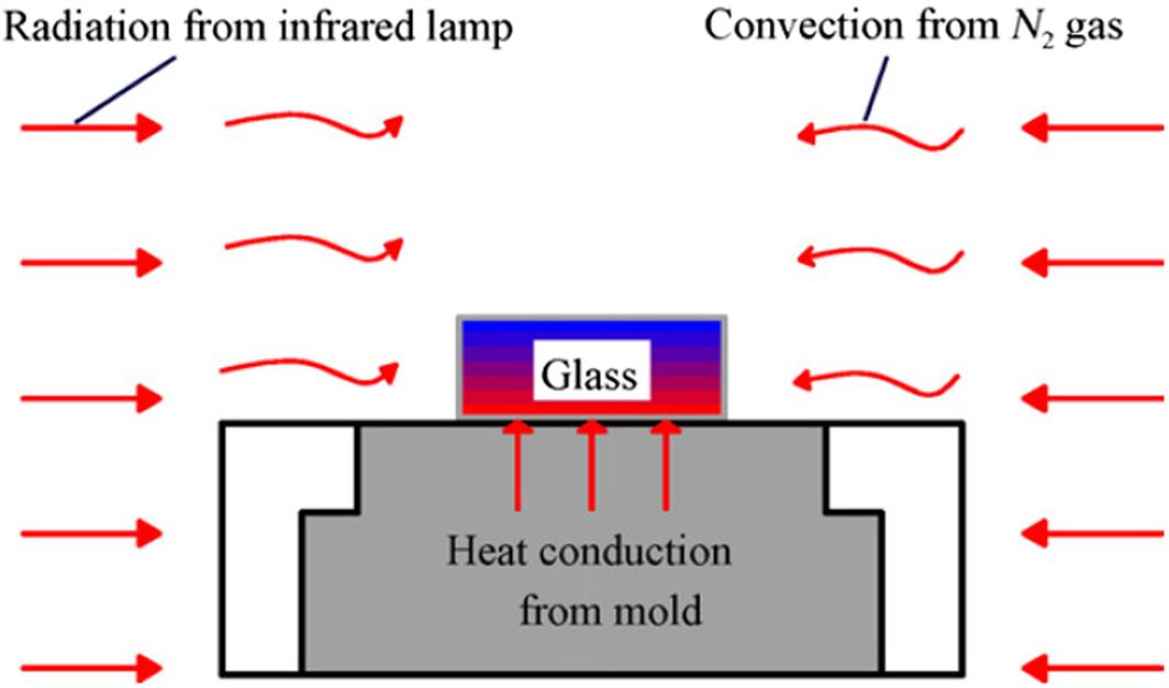
Next, we consider the heat transfer from the mold and the nitrogen environment to the glass preform. As shown in Fig. 8.31, conduction, convection and radiation are three basic modes of heat transfer. In glass molding, thermal conduction at the glass-mold interface and thermal convection between the glass preform and the flowing nitrogen gas are primary contributions to the temperature rise of glass preform. The effect of infrared irradiation on glass is insignificant so that usually it can be ignored, although McGraw (1961) proved that the effect of radiation on the temperature distribution within glass can be described by equivalent thermal conductivity.
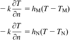
The thermal boundary conditions of the glass preform during heating can be given by Eq. (8.35):
(8.35)
 (8.35)
where ![]() is the interface heat transfer coefficient between the mold and glass;
is the interface heat transfer coefficient between the mold and glass; ![]() is the heat transfer coefficient between the surrounding nitrogen gas and glass;
is the heat transfer coefficient between the surrounding nitrogen gas and glass; ![]() and
and ![]() are the temperatures of the mold and the nitrogen gas, respectively. In Eq. (8.35),
are the temperatures of the mold and the nitrogen gas, respectively. In Eq. (8.35), ![]() is a function of interface pressure, thickness of air gap, amount of sliding, interface temperature, etc., and
is a function of interface pressure, thickness of air gap, amount of sliding, interface temperature, etc., and ![]() is affected by chamber geometry, gas blowing velocity, flowing direction, and so on. Therefore, strictly speaking,
is affected by chamber geometry, gas blowing velocity, flowing direction, and so on. Therefore, strictly speaking, ![]() and
and ![]() are both variables. However, precise measurement of the changes of these coefficients is technically impossible under the present conditions. As a result, like in most of the previous studies (Yi & Jain, 2005), constant values of
are both variables. However, precise measurement of the changes of these coefficients is technically impossible under the present conditions. As a result, like in most of the previous studies (Yi & Jain, 2005), constant values of ![]() (2800 W/(m2K)) and
(2800 W/(m2K)) and ![]() (20 W/(m2K)) are assigned in the FEM simulation.
(20 W/(m2K)) are assigned in the FEM simulation.
High-temperature viscosity of glass
When the temperature is below ![]() , glass is deemed as solid, which can be treated as a rigid or rigid-plastic material. However, when temperature is above the softening point
, glass is deemed as solid, which can be treated as a rigid or rigid-plastic material. However, when temperature is above the softening point ![]() , glass becomes a viscous liquid which is soft and flowable. Between
, glass becomes a viscous liquid which is soft and flowable. Between ![]() and
and ![]() , the properties of glass change greatly with temperature and it behaves as a viscoelastic/plastic body. To achieve glass deformation at a certain load, an experiment is performed near the softening point
, the properties of glass change greatly with temperature and it behaves as a viscoelastic/plastic body. To achieve glass deformation at a certain load, an experiment is performed near the softening point ![]() where glass can be approximately treated as a viscous Newtonian fluid. High-temperature viscosity (
where glass can be approximately treated as a viscous Newtonian fluid. High-temperature viscosity (![]() ) is conventionally measured by parallel-plate viscometers according to Eq. (8.36), as reported by Gent (1960).
) is conventionally measured by parallel-plate viscometers according to Eq. (8.36), as reported by Gent (1960).
(8.36)
where ![]() is the pressing load;
is the pressing load; ![]() is the instantaneous height of the cylindrical glass sample;
is the instantaneous height of the cylindrical glass sample; ![]() is the axial deformation rate; and
is the axial deformation rate; and ![]() is the volume of the sample. Instead of a parallel-plate viscometer, we use an ultraprecision molding machine to measure the viscosity of glass. Two flat molds are used as the rigid parallel-plate pair. Pressing load, displacement and speed are recorded by a load cell and a sensing-control system equipped in the machine.
is the volume of the sample. Instead of a parallel-plate viscometer, we use an ultraprecision molding machine to measure the viscosity of glass. Two flat molds are used as the rigid parallel-plate pair. Pressing load, displacement and speed are recorded by a load cell and a sensing-control system equipped in the machine.
During pressing, glass is assumed to be incompressible. However, the volume of glass will change due to thermal expansion. To improve the accuracy of viscosity measurement, Meister (1982) attempted to make modifications to Eq. (8.30) by considering the thermal expansion. Unfortunately, he made a mistake during formula deduction, which made the modified formula unreliable. Therefore, we correct the formula deduction process as shown in Eq. (8.37).
(8.37)
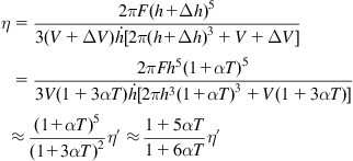 (8.37)
where ![]() is the modified value of viscosity, and
is the modified value of viscosity, and ![]() is the swelling increment in height.
is the swelling increment in height.
After the glass viscosity at certain temperature intervals have been experimentally measured, the viscosity between these temperature intervals can be estimated by curve fitting. The function usually used for fitting glass viscosity is the Vogel–Fulcher–Tamman (VFT) equation as shown in Eq. (8.38) (Fulcher, 1925; Kobayashi, Takahashi, & Hiki, 2006).
(8.38)
where ![]() ,
, ![]() , and
, and ![]() are constants.
are constants.
Stress–strain relationship in viscous deformation
Usually, bulk glass deformation behavior at a low strain rate above yielding point ![]() has been modeled by the Newtonian incompressible law, described in terms of equivalent stress
has been modeled by the Newtonian incompressible law, described in terms of equivalent stress ![]() and strain rate
and strain rate ![]() as given by Eq. (8.39).
as given by Eq. (8.39).
(8.39)
where ![]() is the viscosity of glass, which can be obtained by the VFT equation. However, Chang et al. (2007) found that flow stress function did not follow the exact Newton’s Law for fluids and revised it by modifying the exponent of strain rate based on their experimental results. Similar phenomena is observed. According to the properties of L-BAL42 glass, a modified flow equation is adopted as Eq. (8.40) in the FEM simulation.
is the viscosity of glass, which can be obtained by the VFT equation. However, Chang et al. (2007) found that flow stress function did not follow the exact Newton’s Law for fluids and revised it by modifying the exponent of strain rate based on their experimental results. Similar phenomena is observed. According to the properties of L-BAL42 glass, a modified flow equation is adopted as Eq. (8.40) in the FEM simulation.
(8.40)
It should be mentioned that during pressing, heat transfer still continues. In this case, heat transfers to the glass preform from both the upper and lower molds. However, if the glass preform has been soaked enough so that a uniform temperature distribution is achieved within the glass preform during the heating stage, heat transfer during pressing will be insignificant and will not affect the constants in Eq. (8.40).
The frictional force between glass and molds during pressing is modeled as a constant shear friction (Li, Jinn, Wu, & Oh, 2001), which can be defined by Eq. (8.41).
(8.41)
where ![]() is the frictional stress,
is the frictional stress, ![]() is the shear yield stress, and
is the shear yield stress, and ![]() is the friction factor. In this study, a value of 1.0 is assigned to
is the friction factor. In this study, a value of 1.0 is assigned to ![]() , assuming complete sticking between glass and molds without slip. Under this condition, the friction stress is a function of the yield stress of the deforming glass.
, assuming complete sticking between glass and molds without slip. Under this condition, the friction stress is a function of the yield stress of the deforming glass.
8.3.3.2 FEM simulations
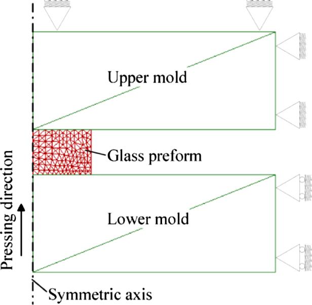
Computer simulations of the glass molding process are carried out using a commercially available FEM program DEFORM™-3D. The program is capable of simulating large deformation of material flow under isothermal and nonisothermal conditions. The FEM model is shown in Fig. 8.32. In the model, the two molds are assumed as completely rigid bodies; the glass preform is deformable and becomes a Newtonian fluid at the pressing temperature. Two-dimensional rigid wall boundaries are used for the upper mold, and one-dimensional rigid wall boundaries are set to the lower mold. The glass preform is totally free of constraints except its surface contact with the two molds. In order to save computation time and improve simulation accuracy, a calculation is done for one-fourth of the cylindrical glass preform by taking advantage of the geometrical symmetry. The element remeshing is updated automatically based on an optimized Lagrangian scheme. The numerical models and boundary conditions and the experimentally measured results of glass viscosity are incorporated into the FEM simulation, which enable a coupled thermal-mechanical analysis.
To start the simulation, the mold is heated from the room temperature to the pressing temperature (590°C). In simulation, the temperature distribution within the molds is assumed to be uniform. The temperature of the lower mold measured by the thermal couple is used as the temperature boundary condition of the mold. Fig. 8.33 shows temperature distributions in the glass preform during heating. After heating for 120 s, the temperature of the bottom surface is 66°C higher than that of the top surface (Fig. 8.33A). The temperature difference is decreased to 10°C after heating for 180 s (Fig. 8.33B). Then, after heating for 220 s, the temperature becomes uniform within the whole glass preform and reach the pressing temperature 590°C (Fig. 8.33C).

Another phenomenon caused by nonuniformity of temperature in glass is that the initially cylindrical glass preform, after pressing, will be deformed to be an isosceles trapezoid where the diameter of the bottom surface is bigger than that of the top surface. Fig. 8.34A shows an example of FEM simulated cross-sectional geometry with strain distribution of a glass piece pressed after a heating time of 180 s. The curvature radius of the upper corner is apparently larger than that of the lower corner. This is due to the fact that the temperature of the upper surface is lower than that of the lower surface in the beginning of press, which cause a higher viscosity at the upper part. Although during pressing the heat transfer from the upper mold can finally eliminate the temperature difference, the deformation of the upper part has been delayed compared to the lower part. This effect finally leads to the trapezoidal geometry of the glass piece. Similarly, in lens molding, nonuniformity of temperature will cause lens form error. Fig. 8.34B shows the equivalent stress (von Mises stress) distribution under the same condition as Fig. 8.34A. The high-stress region is not symmetrical to the horizontal centerline but tends to be lower. This kind of stress distribution may cause deflection of the lens and nonuniformity in its optical properties. Fig. 8.34C shows an instantaneous velocity distribution of element nodes in glass at the end of the first press. It can be seen that near the symmetrical center, velocity vectors are vertically directed; while in the outer region, material flow direction tends to be horizontal. It is also noteworthy that the material in the lower corner is completely stationary at this moment, and material flow can be found only in the upper region.

Fig. 8.35A is a simulated cross-sectional geometry with strain distribution of the glass piece pressed after a heating time of 220 s. In this case, the temperature within the glass has become uniform. The curvature radius of the upper corner of the glass piece is completely the same as the lower corner. Fig. 8.35B shows the corresponding equivalent stress distribution. It is seen that the stress concentration region is basically symmetrical to the horizontal centerline. Fig. 8.35C shows the velocity distribution in the glass at the end of the press. Obviously, velocity vector distribution in the outer region of the glass piece is very uniform, from the upper corner to the lower corner. From this point, we can say that choosing a suitable heating time is not only an important issue for prolonging the service life of molds, but also an essential step for improving form accuracy and optical property of the molded lenses.

High-temperature heat transfer and viscous deformation of glass in a lens molding process have been studied through theoretical analysis and FEM simulations. Thermal expansion and heat transfer phenomena in the glass molding process have been modeled by considering the temperature dependence of thermal properties of glass and interfacial conditions among glass, molds, and environmental gas. The minimum heating time is predicted by FEM simulation. In addition, high-temperature material flow of glass is also simulated by a modified Newtonian fluid model.
8.4 Glass molding process for microstructures
8.4.1 Glass molding machine
In order to conduct glass molding process (GMP) at high temperatures, different molding machine are widely used. There are several commercial machines available, including two main machines that will be discussed below. Both of these machines offer the capability and flexibility required for both scientific research and industrial practice, which enables precise control over the mold position, load, and temperature, while incorporating an extremely flexible design where myriad tests can be accommodated.
8.4.1.1 Glass molding machine PFLF7-60A
The photograph and basic structure and functional features of glass molding machine PFLF7-60A is shown in Figs. 8.36 and 8.37.


The machine is equipped with a drive system, force adaptive control, precision position control and data collection. Some basic adjustment of the machine will be introduced here.
Adjustment of cylinder (see Fig. 8.38)
Cylinder 1 (heating 1)
Cylinder 1 increases the mold temperature with little or without any pressure and it adjusts upward and downward positions by the weight of the cylinder. It is also equipped with two regulators, pressure adjustment and an adjustment for contacting the mold. In this working position, the lens is supposed to be heated to high temperature preliminary and ready for the next position.

Cylinder 2–3 (heating 2–3)
Cylinder 2 and 3 are primarily intended to apply slight pressure and to raise the mold temperature at the same time. So a proper pressure control needs to be done. In these two working positions, the lens is supposed to be heated to the molding temperature.
Cylinder 4 (pressing)
Cylinder 4 is primarily intended to carry out actual molding. It is necessary to perform optimum pressure control on the molds with the lens inside. Cylinder 4 is also equipped with a two-control system consisting of a electro-pneumatic regulator and manual regulator.
Cylinders 5–6 (cooling 1–2)
Cylinders 5 and 6 are primarily intended to apply slight pressure and to lower the mold temperature. In these two working positions, the temperature of lens is supposed to be reduced at a low speed so as to complete the annealing process.
Cylinder 7 (cooling 3)
Cylinder 7 is to decrease the mold temperature with little or without any pressure and the primary purpose is lowering the mold temperature. In this working position, the lens is supposed to be cooled to around 200°.
Other adjustments
Cooling water flow adjustment
The flow rate can be confirmed at a flow rate meter of cooling water. In addition, the cooling water should flow and keep the operating temperature of 20° during heating.
Nitrogen flow adjustment
There is a flow meter that checks the nitrogen pressure and adjusts the nitrogen flow rate with the appropriate value by specific methods. Moreover, nitrogen flows should never stop through the driving time of the heating.
Air adjustment
Each cylinder operating air are managed by one of the original regulator. In addition, it is better to adjust to 0.5 MPa in normal operation.
8.4.1.2 Glass molding machine GMP211
The photograph of glass molding machine GMP211 is shown in Fig. 8.39.

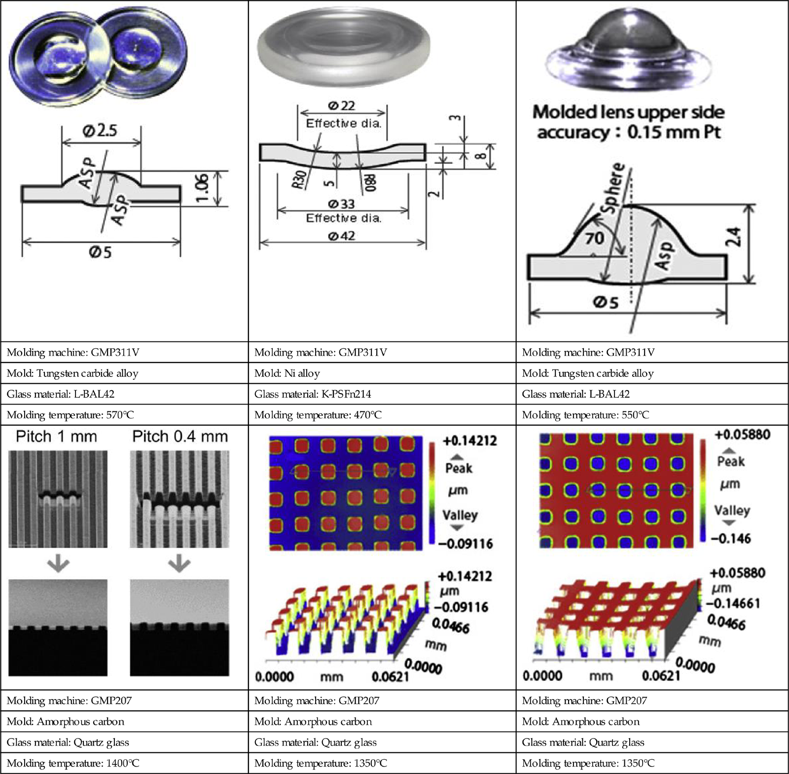
Some typical molded products by glass molding machine from Toshiba Machine Co., Ltd. are shown in Table 8.5.
Table 8.5
Typical molded products from Toshiba Machine Co., Ltd.
 |
 |
 |
| Molding machine: GMP311V | Molding machine: GMP311V | Molding machine: GMP311V |
| Mold: Tungsten carbide alloy | Mold: Ni alloy | Mold: Tungsten carbide alloy |
| Glass material: L-BAL42 | Glass material: K-PSFn214 | Glass material: L-BAL42 |
| Molding temperature: 570°C | Molding temperature: 470°C | Molding temperature: 550°C |
 |
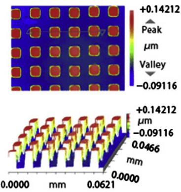 |
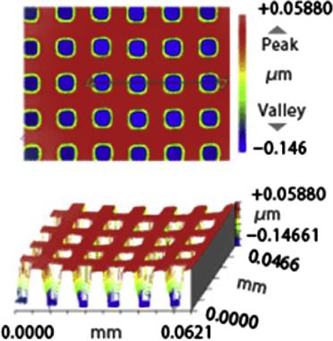 |
| Molding machine: GMP207 | Molding machine: GMP207 | Molding machine: GMP207 |
| Mold: Amorphous carbon | Mold: Amorphous carbon | Mold: Amorphous carbon |
| Glass material: Quartz glass | Glass material: Quartz glass | Glass material: Quartz glass |
| Molding temperature: 1400°C | Molding temperature: 1350°C | Molding temperature: 1350°C |
8.4.2 Molding quality control
8.4.2.1 Temperature control
Glass is a strongly temperature-dependent material. At room temperature, glass is a highly hard and brittle material; at a high temperature, however, it becomes a viscoelastic body or a viscous liquid. Thermal expansion of glass is also significant. For example, the volume-temperature relationship of a commonly used glass L-BAL42 (Ohara Corp., Kanagawa, Japan) is plotted in Fig. 8.40. Softening point (![]() ) is defined as the temperature at which the glass deforms under its own weight and behaves as liquid. Yielding point (
) is defined as the temperature at which the glass deforms under its own weight and behaves as liquid. Yielding point (![]() ), also called “deformation point,” is a temperature at which glass reaches its maximum expansion and a relatively low plasticity and starts shrinking. When such a melt is gradually cooled, the volume decreases abruptly down to a transition temperature (
), also called “deformation point,” is a temperature at which glass reaches its maximum expansion and a relatively low plasticity and starts shrinking. When such a melt is gradually cooled, the volume decreases abruptly down to a transition temperature (![]() ) below which volume shrinkage occurs at a slower rate. Pressing of a glass lens is always performed above
) below which volume shrinkage occurs at a slower rate. Pressing of a glass lens is always performed above ![]() . Annealing point (
. Annealing point (![]() ) is the upper end of the annealing range for the pressed glass lens, at which the internal stress is reduced to a practically acceptable value over a short period. Strain point (
) is the upper end of the annealing range for the pressed glass lens, at which the internal stress is reduced to a practically acceptable value over a short period. Strain point (![]() ) represents the lower end of the annealing temperature range. It is also the upper limit of service temperature of a glass component. During annealing, glass is slowly cooled down from
) represents the lower end of the annealing temperature range. It is also the upper limit of service temperature of a glass component. During annealing, glass is slowly cooled down from ![]() to somewhat below
to somewhat below ![]() .
.

 , softening point;
  , yielding point;
  , transition point;
  , annealing point;
  , strain point.
Determination of a suitable temperature for pressing is an essential issue for glass molding. If pressing is performed above ![]() and held on to keep the shape of the lens during cooling, the volume expansion around
and held on to keep the shape of the lens during cooling, the volume expansion around ![]() will lead to a sharp increase in pressing load, and in turn, adhesion of glass to molds. On the contrary, if pressing is done below
will lead to a sharp increase in pressing load, and in turn, adhesion of glass to molds. On the contrary, if pressing is done below ![]() , a high pressing load will be required since glass is not sufficiently softened at this temperature range. In this case, significant residual stresses will occur in the glass lens, and the high pressing load may also shorten the service life of the molds. This problem is a critical one especially when molding micro Fresnel lenses and DOEs where the molds have extremely fine grooves on the surface. Therefore a suitable temperature for pressing is truly necessary in glass molding process for microstructures.
, a high pressing load will be required since glass is not sufficiently softened at this temperature range. In this case, significant residual stresses will occur in the glass lens, and the high pressing load may also shorten the service life of the molds. This problem is a critical one especially when molding micro Fresnel lenses and DOEs where the molds have extremely fine grooves on the surface. Therefore a suitable temperature for pressing is truly necessary in glass molding process for microstructures.
8.4.2.2 Mold oxidation prevention
In a lens molding process, a glass blank or gob is initially heated to a temperature above its transition and subsequently pressed between the two mold halves into a lens shape. During the whole molding process, especially the heating and pressing process, the glass and mold must be heated in oxygen free environment to prevent oxidation that may damage the surface quality of glass and reduce the service life of mold.
In present glass molding machines, they generally offer two approaches to isolate from oxygen. One is a vacuum environment and the other is a nitrogen environment. For instance, glass molding machine GMP211 by Toshiba Machine Co., Ltd. provides a vacuum environment to fabricate the lens, while glass molding machine PFLF7-60A by SYS Co., Ltd. offers a nitrogen environment. There are advantages and disadvantages in both methods to avoid oxidation, as shown in Table 8.6.
8.4.2.3 Methods to increase mold life
Improve pressing method
Some steps can be added into the molding process to increase the mold life in condition of no bad effect on form accuracy. Based on the conventional method, we propose a two-step pressing method. The first pressing step is done at a high temperature near the softening point (![]() ), so that glass behaves as a viscous liquid and most of the material deformation can be achieved at a low load. After the first step, the pressing load is reduced and the temperature is lowered to be between
), so that glass behaves as a viscous liquid and most of the material deformation can be achieved at a low load. After the first step, the pressing load is reduced and the temperature is lowered to be between ![]() and
and ![]() . Then the second pressing is done at this temperature to close the molds and obtain the final shape of the lens. This two-step pressing method can achieve both high lens accuracy and long mold life.
. Then the second pressing is done at this temperature to close the molds and obtain the final shape of the lens. This two-step pressing method can achieve both high lens accuracy and long mold life.
Coating
One crucial requirement of a mold for glass lenses is the demolding ability. That is to say, the finished lens must be easily removed from the molds. In high-temperature glass molding, the surface of the mold tends to oxidize and the oxidized material diffuses into the glass, causing adhesion of the glass lens to the mold. Therefore, a release agent is usually coated onto the surface of the mold to prevent oxidation. It is generally considered that the lifetime of a mold is almost completely determined by that of the release agent coating. Wearing and flaking of this coating reduces the lifetime of the mold. Moreover, deterioration of the oxidation resistance of the release agent due to in-diffusion of elements from the mold leads to an increased level of wettability by the glass which again reduces the mold lifetime. Thus, the lifetime of the mold is influenced both by interactions between the release agent and the mold and the release agent and the glass. Consequently, the choice of an appropriate release agent for the mold substrate is critical.
Mold equipment diagnosis techniques
As for the measures to achieve the long life of mold, there is an improvement in software in addition to the aforementioned improvements in hardware. The improvement in software mentioned here means application of an equipment diagnosis technique to find out the deterioration of equipment quantitatively, predict mold life up to the allowable criterion, and replace the mold at the proper timing just before the criterion is reached.
8.4.3 Molding defects
8.4.3.1 Incomplete filling
Conventionally, the accuracy is low in microgroove forming due to the incomplete filling of the material in the cavity of microgroove mold. It makes incomplete filling become one of most important molding defects in the glass molding process. When the stress applied to the material sample is constant, the dashpot representing Newtonian fluid features plays a dominant role during deformation. The energy loss caused by Newtonian fluids reduces the filling rate after a period of deformation because the material flow rate decreased by time.
We should look into the reasons for the forming error of the molded microstructures. First, the GMP is carried out at a high temperature of 570°C. After pressing, the formed microstructure arrays are cooled to room temperature. The formed microstructures will contract and reduce the filling ratio. Therefore, a low molding temperature is preferred in the microstructure forming for higher filling ratio of glass.
The filling ratios of the glass at different friction coefficients are studied here by using a commercial FEM code ABAQUS. We can see from Fig. 8.41 that the filling ratios of the glass tend to become lower with the declining of a friction coefficient. Therefore, it is appropriate to avoid the incomplete filling by increasing the friction coefficient between glass and molds.
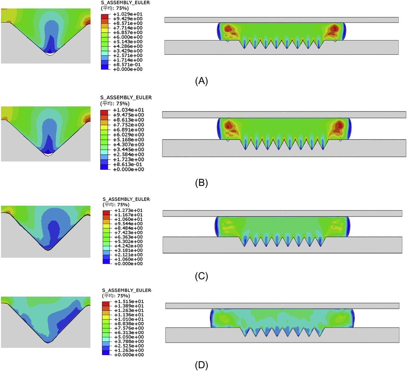
8.4.3.2 Surface defects
Wrinkles
Microgrooves were fabricated by a hot pressing process. Fig. 8.42A is the SEM photograph of the microgrooves pressed without ultrasonic vibration, and Fig. 8.42B is the SEM photograph of the microgrooves fabricated by ultrasonic vibration assisted pressing. We can find that many irregular wrinkles appear on the slope surface of the microgrooves, especially near the valleys of the microgrooves, which is consistent with stress concentration area appears in FEM simulation, when they are pressed without ultrasonic vibration. When ultrasonic vibration is applied, wrinkles almost disappear, and a smooth surface is achieved.

Dents and pores
There are some dents and pores on the surface of aspherical lenses, as shown in Fig. 8.43. The possible reasons could be various, including improper molding temperature and molding pressure. Also, it could be caused by the defect on molds. Fig. 8.44 shows the SEM photographs of microgrooves with side burrs at different magnifications. The shape errors or other surface defects of the microstructures on the mold fabricated by microcutting can be easily replicated to the microstructures on the glass surface in the GMP process. Therefore, the shape accuracy and surface defects of the microstructures on the mold should be precisely generated above all.


Glass adhesion
Fig. 8.45 shows the micrographs of microgrooves on the mold before GMP and after GMP. It is clear from the figure that some glass material has adhered to the molds. Process conditions during glass molding such as high temperature, long contact time and high mechanical load often lead to strong adhesion between the inorganic glass piece and the molds. This sticking behavior that could result in the surface quality deterioration of the molds and potentially destroy the mold has not been properly understood. The majority of the discrepancies can be attributed to the lack of proper understanding of the glass-mold interaction (Fischbach et al., 2010).
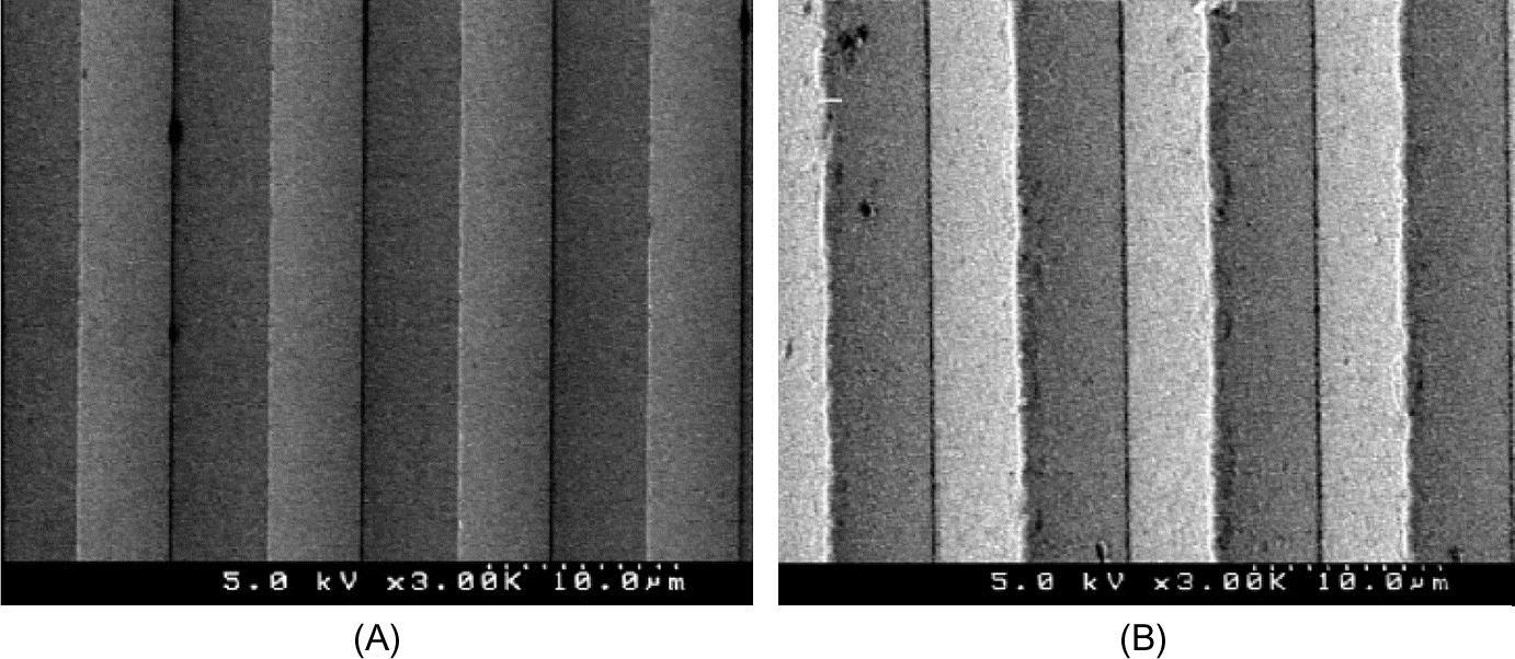
Experiments were performed to search for how glass-mold interfaces impact sticking in glass mold systems. It shows that the sticking of glass to the mold can be partially controlled by three methods: decreasing surface roughness value, lubricating the surface, and pre-oxidizing the surface. In the case of precision glass molding, lubrication and increased surface roughness cannot be used to reduce the sticking force because of the very nature of high surface quality required for optical performance. Some attempts are made to create a new testing method for hot forming processes where the characterization of the sticking behavior of mold materials and coatings is possible and the corrosion and wear behavior of mold material can be quantified. The sticking characteristics of the molds and coatings could be described by the “lower” and the “upper” sticking temperatures. Although the results of their experiment appear to be valid, the use of molten glass is a significant deviation from the process conditions associated with precision glass molding, where the glass never reaches its melting temperature but remains a viscoelastic solid throughout the process.
8.5 Summary
This chapter mainly introduces the glass molding process (GMP) for microstructures, which include microgrooves, micropatterns, microprisms and microlenses. It describes the basic working principle of microstructures in many fields as well as the fundamentals of glass molding techniques. This chapter mainly concentrates on modeling and simulation of microstructure molding process and offers specific methods to conduct simulation calculations of coupling heat transfer and viscous deformation. Also, some typical problems, such as molding quality control and molding defects prevention in the glass molding process, are discussed in detail.