1.2.1 Minimum chip thickness and size effect

The set-up used in the modeling of microscale cutting is similar to the one used in the macroscale traditional cutting processes (i.e., a wedge-like tool is removing material from a surface). All the geometrical features and kinematic characteristics of the tool and workpiece are identifiable. However, downscaling all phenomena in order to apply the same theories in both the micro and macro regime proves to be inadequate. There are features of machining and phenomena that are considerably different in micromachining and do not allow for such a simplification. These differences arise when considering the chip formation process, the resulting cutting forces, the surface integrity, and tool life.

In Fig. 1.1, the orthogonal cutting model corresponding to microscale cutting may be observed. At this level, the depth of cut may be well below 10 μm with an anticipated surface roughness of only a few nm. The cutting edge, no longer be considered sharp, has a cutting edge radius comparable in size to the uncut chip thickness. Although the rake angle of the tool indicated in Fig. 1.1 is positive, the actual the effective rake angle participating in the processes is negative. In this case, the elastic-plastic deformation of the workpiece material and ploughing need to be taken into account, as well as the elastic recovery at the clearance face.

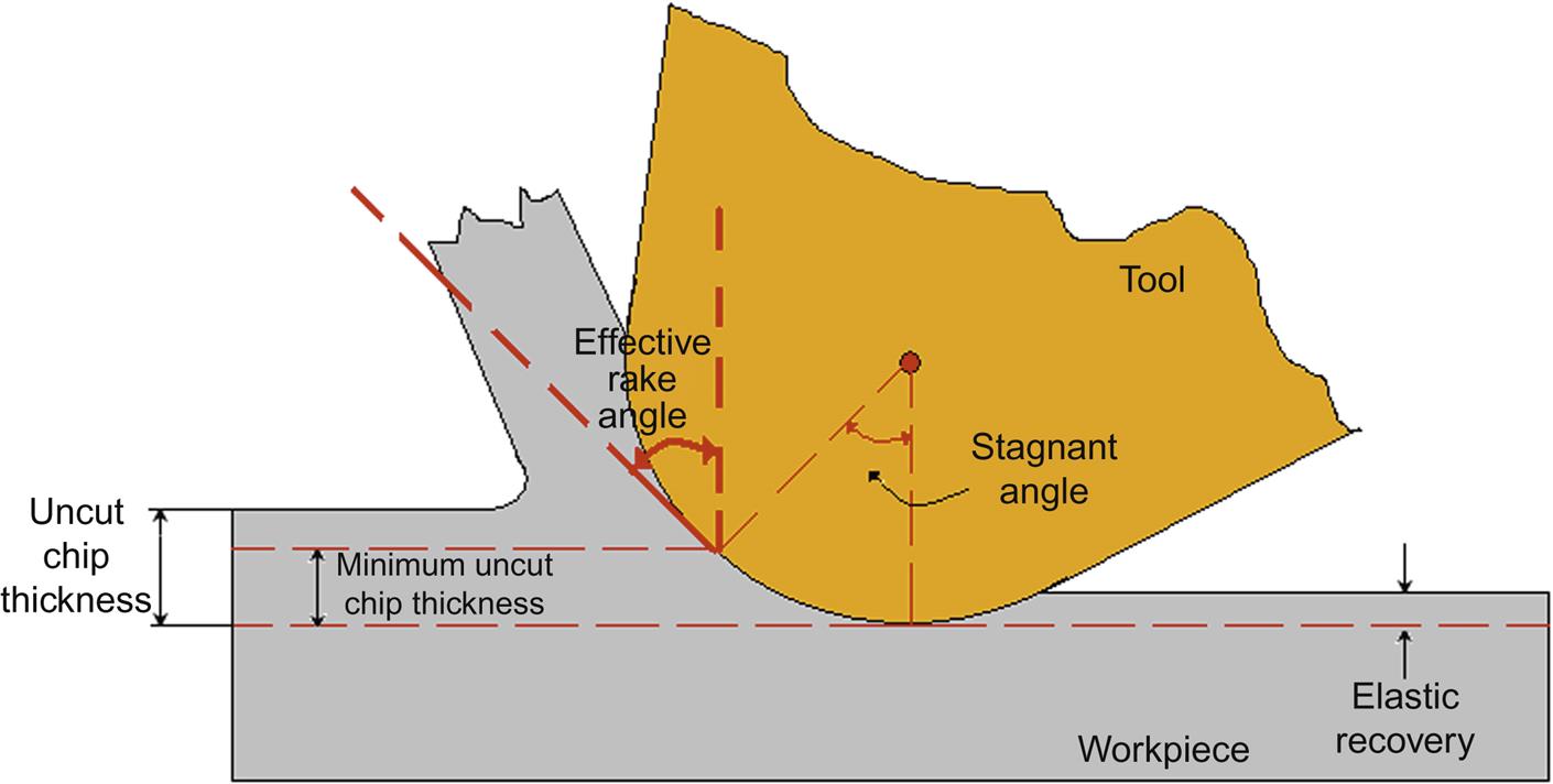
As explained above, one may deduct the existence of a removable minimum chip thickness from the workpiece surface in a mechanical micromachining operation. A stagnation point above which a chip is formed and below only elastic-plastic deformation takes place is assumed. The stagnation point is connected to a stagnant angle θ_m, which with the tool edge radius determines the value of the minimum uncut chip thickness, h_m (Malekian, Mostofa, Park, & Jun, 2012):

$h_{\mathrm{m}}=r_{\mathrm{e}}(1-\cos {\theta }_{\mathrm{m}})$ (1.1)

(1.1)

The minimum chip thickness determines whether a chip is formed or not, because if the depth of cut for a microcutting operation is set below this minimum, then the cutting edge is expected to plastically deform the workpiece material without producing a chip. This is known as the ploughing mechanism. In addition to the obvious effect on the surface integrity and quality of the finished workpiece, it significantly alters the cutting forces, and thus the process stability, in microscale machining and makes the force prediction methods ineffective. The minimum chip thickness was identified in grinding by Finnie (1963) and also in microturning and micromilling by several other researchers. Ikawa, Shimada, Tanaka, and Ohmori (1991), using a turning diamond tool with an edge radius of about 10 nm, found the uncut chip thickness is approximately 1/10 the cutting edge radius. Weule, Huntrup, and Tritschle (2001) studied the minimum chip thickness for micromilling. In this case, during the same pass of a cutter’s single tooth from the workpiece on a chip of varying thickness, the material removal mechanism may change from shearing to ploughing or vice versa, resulting in a saw tooth-like surface profile and a deteriorating surface finish. The minimum chip thickness was also reported in micromilling by Kim, Bono, and Ni (2002) by comparing the process with nominal chip volume and the workpiece surface feed marks with the feed per tooth. It was concluded that a chip was not formed with every pass of a cutting tooth, and this was attributed to the minimum chip thickness.

Although ploughing may exist in machining, the study of its effect on the overall process may be neglected. The effect caused by the cutting edge radius is important in microscale cutting. Many researchers consider this to be the primary cause of the size effect, the nonlinear increase in the specific energy, and the specific cutting force with decreasing depth of cut, all of which are observed in microcutting. Albrecht (1960, 1961) argues that there are two areas where ploughing occurs, one on the rake face and another around the tool edge. Masuko (1956) introduces a new effect that acts independently from ploughing and calls it indenting. According to this theory an indenting force causes the cutting edge to penetrate the workpiece; this force is held responsible for the size effect according to this theory.

The size effect was identified in metal cutting operations as early as 1952 by Backer et al. The researchers processed specimens made of SAE 1112 steel with grinding, micromilling, turning, and tension tests. These data correlate chip thickness with resisting shear stress, and clearly show the size effect, which is attributed to the significantly reduced amount of imperfections—namely crystallographic defects such as grain boundaries, missing and impurity atoms, and inhomogeneities present in all commercial metals—encountered when deformation takes place in a small volume. With smaller uncut chip thickness, the material strength is expected to reach its theoretical value of strength. Many more investigators have acknowledged the size effect experimentally and theoretically (Kim & Kim, 1995).

Although size effect, such as minimum chip thickness, is present in metal cutting, it is of special importance in microscale cutting. Aside from the explanations already mentioned, there are several other discussions regarding the size effect appearance. It is also attributed to material strengthening due to increasing the strain rate in the primary shear zone (Larsen-Basse & Oxley, 1973) or to decreasing temperature in the tool-chip interface (Kopalinsky & Oxley, 1984) with decreased chip thickness. Atkins (2003) proposes that the size effect is due to the energy required for new surface creation via ductile fracture. Another explanation is based on the size effect appearing in micro-nano-indentation and its extension to machining (Dinesh, Swaminathan, Chandrasekar, & Farris, 2001). The increased hardness of a material with reduced indentation depth is a result of the dependence of material flow stress on the strain gradient in the deformation zone; strain gradient plasticity can be the reason of size effect in machining because of the intense strain gradients observed. The criticism of this theory stems from the fact that the size effect’s impact on hardness in indentation is related to size effect in cutting when the von Mises criterion is applicable. However, this assumption is not compatible with the experiments of Merchant (Shaw & Jackson, 2006). However, some works using analytical and FEM models and experimental validation based on strain gradient plasticity have been published (Joshi & Melkote, 2004; Liu & Melkote, 2007).

From the literature review, it is evident that many reasons for the size effect in machining and microscale cutting have been reported. It is not clear which of the above mechanisms is dominant, or whether there could be more than one mechanism acting simultaneously. Even when multiple mechanisms act together, there may be additional influences that alter the contribution of each factor in each case. For further reading on the size effect in machining, and especially in micromachining, the works of Liu, DeVor, Kapoor, & Ehmann (2004), Shaw (2003), and Shaw & Jackson (2006) are suggested.

1.2.2 FEM modeling of microscale cutting

In this section, the aspects of modeling microscale cutting with FEM are explored. FEM modeling of machining presents similarities in its macro- and micro-scale forms. General examples of FEM applications in manufacturing technology, and in particular, cutting, can be found in the works of Dixit & Dixit, 2008; Klocke et al., 2002; Mamalis, Manolakos, Ioannidis, Markopoulos, and Vottea, 2003. The following paragraphs provide a detailed description of the modeling of cutting, with focus on the modeling of microscale cutting.

1.2.3 FEM basics

In FEM, the basic principle is discretization (i.e., the replacement of a continuum by finite elements forming a mesh). Each finite element is simpler in geometry and therefore easier to analyze than the actual structure. Every finite element possesses nodes where the initial problem and boundary conditions are applied, and the degrees of freedom are calculated. Furthermore, the finite elements are connected to one another in nodes. The problem variables as well as properties applied on the nodes of each element are assembled, and global relations are formatted.

Two different time integration strategies address nonlinear and dynamic models. These refer to implicit and explicit schemes. The former approach solves the set of finite element equations by using a central difference rule to integrate the equations of motion through time. While the latter is realized by solving the set of finite element equations and performing iterations, until a convergence criterion is satisfied for each increment. Another topic pertains to the use of a certain numerical formulation. Currently, the ones used in metal cutting FEM models are of three types: Eulerian, Lagrangian, and the newer arbitrary Lagrangian-Eulerian (ALE) analysis. In the Eulerian approach, the finite element mesh is spatially fixed and covers a control volume where the material flows through it in order to simulate the chip formation. In the Lagrangian approach, the elements are attached to body-centered meshes (e.g., that of the workpiece). The workpiece is deformed due to the action of the cutting tool, and consequently so is the mesh, providing a more realistic simulation. Disadvantages of the Lagrangian formulation is connected to the large mesh deformation observed during the simulation and the use of chip separation criteria. The updated Lagrangian analysis has overcome the disadvantage of a chip separation criterion by applying continuous re-meshing and adaptive meshing, dealing at the same time with the mesh distortion. Finally, the ALE formulation has also been proposed with the aim to combine the advantages of the two aforementioned methods. More details on the subjects discussed in this paragraph can be found in the work of Markopoulos (2013).

1.2.4 FEM cutting models

As expected, the geometrical characteristics of the tool and the workpiece greatly influence the outcome of the microscale cutting models. Specifically, the tool edge radius is connected to the size effect, minimum chip thickness, effective rake angle, stagnation point, and ploughing mechanism, as discussed in the previous section. In microcutting, the simulation of the process with a sharp tool is of no interest because the size effect would not be accounted for; the size of the cutting forces and the chip formation would be unrealistic. Some researchers have investigated the influence of the tool edge radius on the size effect. Weber et al. (2007) performed an analysis using similarity mechanics and various values for the tool edge radius. Woon, Rahman, Neo, and Liu (2008) also investigated the tool edge radius and its influence on the material deformation and the contact length between the tool and workpiece and then validated their numerical results with the aid of a small field-of-view photography technique. Liu and Melkote (2007) concluded from their analysis that the tool edge radius accounts for only part of the size effect in microcutting, and the material strengthening is associated with a temperature drop in the secondary deformation zone for higher cutting speeds.

Another topic of interest pertains to the boundary conditions applied in the initial mesh, and specifically, the manner thermo-mechanical coupling is considered. In cutting processes, heat generation originates from the two deformation zones (i.e., the primary and the secondary) due to inelastic and frictional work. Addressing this problem involves a nonlinear analysis of the associated strain hardening and thermal softening in these zones. This feature of the model is important for microscale cutting, since the size effect is attributed to material strengthening due to a temperature decrease in the tool–chip interface with a decreased chip thickness (Kopalinsky & Oxley, 1984).

Moriwaki, Sugimura, and Luan (1993) developed a thermo-mechanical model of copper micromachining and calculated the stress, strain flow of the cutting heat, and temperature of the tool and the workpiece. Effective strain hardening and thermal softening are integrated by employing tribological and material models that are functions of mechanical and thermal behavior with strain, strain-rate, and temperature.

1.2.5 Friction modeling

Microscale cutting uses the same assumptions as macroscale cutting, regarding the secondary deformation zone in friction modeling at the interface of the chip and rake face of the tool. Many researchers utilize Coulomb’s law (i.e., the frictional sliding force is proportional to the applied normal load, and the ratio of these two is the coefficient of friction μ which is constant in all the contact length between chip and tool). The relation between frictional stresses τ and normal stresses may be expressed as:

$\tau =\mu \sigma$ (1.2)

(1.2)

However, as the normal stresses increase and surpass a critical value, this equation fails to give accurate predictions. Experimental analysis verifies that two contact regions may be distinguished in dry machining, namely the sticking and sliding regions. Zorev’s (1963) stick-slip temperature independent friction model is the one commonly used. In this model, there is a transitional zone with distance _c from the tool tip that signifies the transition from sticking to sliding regions. Near the tool cutting edge and up to _c (i.e., the sticking region), the shear stress is equal to the shear strength of the workpiece material, k; while in the sliding region, the frictional stress increases according to Coulomb’s law.

$\tau =\{\begin{array}{l}k,0\le \ell \le {\ell }_{\mathrm{c}}\hfill \\ \mu \sigma ,\ell >{\ell }_{\mathrm{c}}\hfill \end{array}$ (1.3)

(1.3)

In machining based on Zorev’s model, other approaches have been reported that include the defining of an average friction coefficient on the rake face or different coefficients for the sliding and sticking regions (Childs & Maekawa, 1990; Iwata, Osakada, & Terasaka, 1984; Sekhon & Chenot, 1993; Usui, Maekawa, & Shirakashi, 1981; Yang & Liu, 2002). For more information on friction models in cutting, the reader is encouraged to read the work of Markopoulos (2013).

1.2.6 Material modeling

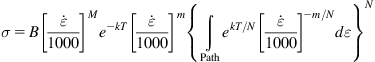
Material modeling in microscale machining is of particular interest, especially the extensively studied flow properties of the workpiece material and the corresponding equations included in FEM. These constitutive equations describe the flow stress or instantaneous yield strength at which work material starts to plastically deform or flow. Some of the many constitutive equations employed in metal cutting are discussed here. The first is the relation by Usui et al. (1981):

$\sigma =B{\left[\frac{\stackrel{·}{\epsilon }}{1000}\right]}^M{e}^{-kT}{\left[\frac{\stackrel{·}{\epsilon }}{1000}\right]}^m{\left\{\underset{\mathrm{Path}}{\overset{}{\int }}{e}^{kT/N}{\left[\frac{\stackrel{·}{\epsilon }}{1000}\right]}^{-m/N}d\epsilon \right\}}^N$ (1.4)

(1.4)

In this equation, B is the strength factor, M is the strain-rate sensitivity, N the strain hardening index, all functions of temperature are T, and k and m are constants. The integral term accounts for the historical effects of strain and temperature in relation to strain rate. In the absence of these effects, the last equation is reduced to (Childs, Otieno, & Maekawa, 1994):

$\sigma =B{\left[\frac{\stackrel{·}{\epsilon }}{1000}\right]}^M{\epsilon }^N$ (1.5)

(1.5)

Among the most used material models is the Johnson–Cook model (1983). The equation consists of three terms: the elasto-plastic term represents strain hardening, viscosity demonstrates that material flow stress increases for high-strain rates, and the temperature softening term for the softening of the material due to temperature increase. It is a thermo-elasto-visco-plastic material constitutive model described as:

$\sigma =\left(A+B{\epsilon }^n\right)\left[1+C\ln \left(\frac{\stackrel{·}{\epsilon }}{{\stackrel{·}{\epsilon }}_{\mathrm{o}}}\right)\right]\left[1-{\left(\frac{T-T_{\mathrm{a}}}{T_{\mathrm{m}}-T_{\mathrm{a}}}\right)}^m\right]$ (1.6)

(1.6)

where T_a is the ambient temperature; T_m the melting temperature; and A, B, C, n, and m are constants that depend on the material and are determined by material tests (Jaspers & Dautzenberg, 2002; Lee & Lin, 1998) or predicted (Özel & Karpat, 2007). Umbrello, M’Saoubi, and Outeiro (2007) investigated the influence of the Johnson-Cook constants on the outcome of machining modeling and found that FEM results are sensitive to these inputs, which in turn are strongly related to the test method used to derive the constants. On the other hand, the results from a test method can be plugged into different constitutive equations, and the selection of the material model can influence the predicted results (Liang & Khan, 1999; Shi & Liu, 2004). A review of material models used in manufacturing processes, including microcutting, can be found in the work of Dixit, Joshi, and Davim (2011).

All the above mentioned FEM material models refer to isotropic materials. No crystallographic effects are considered in the modeling process. Zerilli and Armstrong (1987) developed a constitutive model based on dislocation-mechanics theory and consideration of materials’ crystal structures. They suggested two different models, one for body-centered cubic(BCC) and the other for face-centered cubic (FCC) lattice structure, respectively:

$\sigma =C_{\mathrm{o}}+C_1\exp [-C_{3}T+C_{4}T\ln (\stackrel{·}{\epsilon })]+C_5{\epsilon }^n$ (1.7)

(1.7)

$\sigma =C_{\mathrm{o}}+C_2{\epsilon }^n\exp [-C_{3}T+C_{4}T\ln (\stackrel{·}{\epsilon })]$ (1.8)

(1.8)

where C_i, i=0–5, and n are material constants determined experimentally (e.g., by the SHPB method) (Meyer & Kleponis, 2001).

In microscale cutting, the cutting tool radius is comparable to the size of the grains of the material being processed. Furthermore, in materials with surface defects or multiphase materials, such as cast iron, the microcutting mechanism is quite different in comparison to nonheterogeneous materials due to the encounter of the cutting tip with these features of the material during the course of the process. The model prepared by Chuzhoy, DeVor, and Kapoor (2003) simulates cutting at a microstructure level. Ductile iron and two of its constituents, namely pearlite and ferrite, are modeled in the same continuum, taking into account the microstructural composition, the grain size, and the distribution of each material. The model’s position of predict stresses, strains, and temperatures. Simoneau, Ng, and Elbestawi (2006a, 2006b, 2007a, 2007b) studies involve the machining of 1045 steel and consider its microstructure. In their models, the initial mesh of the material is divided into bands of material A, with a pearlite-like behavior, and bands of material B, with a ferrite-like behavior; the material bands are of appropriate size. Material plasticity is formulated with a strain dependent Johnson-Cook model. The results of the analysis show good correlation between experimental and numerical results regarding the morphology of the chip and the behavior of each phase of the material. The predicted strain result was larger in a heterogeneous FEM model in comparison to a homogeneous one due to strain localization at each phase.

However, when nanoscale cutting is considered, material modeling cannot be adequately represented by continuum mechanics; a more detailed view on the materials microstructure and the interaction between the workpiece, the tool, and the chip is required. For this reason, the MD method, presented in detail in the next part, is applied for cutting process simulation at this scale.

1.3.1 Model geometry and material microstructure

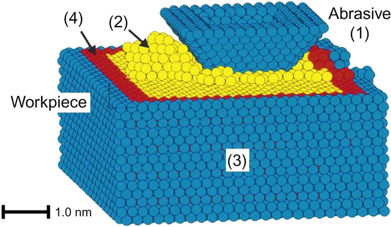
One of the most fundamental subjects in simulations is the accurate description of the geometric entities that constitute the domain on which the solution of governing equations is required. Realistic geometric modeling can produce more reliable results, if combined with the appropriate material properties, boundary conditions, and other numerical details, and is required in order to conduct comparisons with experimental studies. Fig. 1.3 depicts a general model set-up, resembling orthogonal cutting, which is often used in MD simulations.

The majority of workpiece geometry cases are simplistic and have the form of a rectangular box. Usual sizes extend up to several tenths of nanometers, depending on the material type, and the number of atoms is in the order of 10⁵. It is noteworthy to mention that due to the direct correlation of model size to computational requirements, model sizes are restricted by the available computational power. However, cases exist in the literature where models with almost a million atoms are reported (Ren, Zhao, Dong, & Liu, 2015; Tong, Liang, Jiang, & Luo, 2014). Also, multimillion atom models were created in order to study, among other topics, the effect of workpiece size on the results of the simulation (Pei, Lu, & Lee, 2007; Xiao, To, & Zhang, 2015). Large-scale MD simulations with model sizes up to ten million atoms can also be found in the literature (Pei, Lu, Lee, & Zhang, 2009). The arrangement of the atoms in workpiece strictly follows the atomic structure of each material. On rare occasions (Eder, Bianchi, Cihak-Bayr, Vernes, & Betz, 2014; Li, Fang, Zhang, & Liu, 2015; Rashid, Goel, Luo, & Ritchie, 2013), a modified type of the surface is used as the effect of surface roughness on the outcome of the machining process is desired. Moreover, the material can be modeled as a multigrain bulk or various crystal orientations may exist in the workpiece (Goel, Luo, Reuben, & Pen, 2012; Junge & Molinari, 2014; Solhjoo & Vakis, 2015). Furthermore, there are some rare cases where lubricants or cutting fluids are taken into consideration in the simulation (Chen, Cian, Yu, & Huang, 2014; Ren et al., 2015; Rentsch & Brinksmeier, 2005; Rentsch & Inasaki, 2006). Obviously, knowledge of crystal structures is fundamental when modeling a workpiece in MD simulations. Crystal structures are considered as unique arrangements of atoms, molecules, or atoms within a crystalline material. The most common lattice systems employed in nanocutting atomistic simulation are BCC, FCC, and body-centered tetragonal, which correspond to the most common engineering materials.

Tool geometry is generally somewhat more complex and diverse than the workpiece geometries. The majority of nanomanufacturing simulations involve the use of a cutting tool as they represent general nanocutting processes. Usually, the tool shape is process-dependent; the tool is portrayed as close as possible to a real cutting tool. In many cases, the cutting tool is considered rigid, and the tool atoms retain their relative positions while travelling at constant speed relative to the workpiece. The simplest form of cutting tool has a round or atomically sharp edge (Gao et al., 2009; Lin, Lin, & Hsu, 2014; Rentsch & Brinksmeier, 2005), and its geometric representation includes the definition of rake and clearance angles. Studies with various rake angles are also conducted (Markopoulos, Karkalos, Kalteremidou, Balafoutis, & Manolakos, 2015a; Pei, Lu, Fang, & Wu, 2006), even with negative ones (Komanduri, Chandrasekaran, & Raff, 1999). Furthermore, in nanogrinding simulations, the cutting tool is represented as having single (Markopoulos, Savvopoulos, Karkalos, & Manolakos, 2015b; Rentsch & Inasaki, 1994; Rentsch & Inasaki, 1995) or multiple grains with a cubic (Brinksmeier et al., 2006), ellipsoid (Eder et al., 2014), or spherical shape (Li, Fang, Liu, & Zhang, 2014).

1.3.2 Potential function

Potential functions are employed in MD simulations as means of representing material behavior at the atomistic scale. A variety of potential functions has been developed during the past decades with a view to simulate interaction between atoms of the same or different type. Historically, Lennard-Jones and Morse potentials were the first to be employed. However, over time, more complex potentials, such as embedded atom method (EAM) potential or bond-order potentials, are developed with significantly better accuracy. All of these potentials involve the determination of a set of parameters, calculated either from experimental findings or from simulations with more fundamental methods. When the potential function is selected, force can be directly calculated, as the first derivative of potential energy with respect to position.

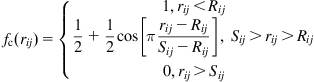
The Lennard-Jones potential is a simple simulation model describing interaction between a pair of uncharged atoms or molecules as a function of the distance between their centers. Its most common expression is the so-called 12-6 Lennard-Jones potential:

$V=4\epsilon \left[{\left(\frac{\sigma }{r}\right)}^{12}-{\left(\frac{\sigma }{r}\right)}^6\right]=\epsilon \left[{\left(\frac{r_{\mathrm{m}}}{r}\right)}^{12}-2{\left(\frac{r_{\mathrm{m}}}{r}\right)}^6\right]$ (1.9)

(1.9)

where ε is the energy constant (or well depth, depicting interaction strength), σ is effectively the diameter of one of the atoms (or the distance at which the two particles are at equilibrium), and r_m represents the distance when potential energy is minimum and is equal to 2^1/6σ. The Lennard-Jones potential curve is depicted in Fig. 1.4.

The Lennard-Jones potential is considered a good approximation for a preliminary study of an atomistic system, and is particularly sufficient in modelling noble gases. Lennard-Jones potential assumes that interactions are valid for an infinite range. Although the interatomic forces fade over a large distance, the definition of a cut-off distance is necessary to reduce the unnecessary computational cost for calculations between atoms separated by a large distance. The cut-off distance is often set at 3σ. In terms of nanoscale cutting, Lennard-Jones potential is rarely employed (Eder et al., 2014; Oluwajobi & Chen, 2011a), especially in cases where potential functions do not exist for a material or to model a more complex material, as in Solar et al. (2011).

Morse potential is another two-body potential function for the calculation of interatomic interactions. This potential function provides a good approximation of molecular vibration (vibrational excitations of a chemical bond). It is considered the simplest potential function that can simulate dissociation between two atoms, which would be impossible to be simulated with a harmonic oscillator model. Morse potential has a simple formulation and requires the definition of only three parameters to provide the potential energy of a diatomic molecule:

$V=D_{\mathrm{e}}\left(e^{-2a(r-r_{\mathrm{e}})}-2e^{-a(r-r_{\mathrm{e}})}\right)$ (1.10)

(1.10)

where r is the distance between the atoms (or internuclear distance), r_e is the equilibrium bond distance (bond length), D_e is the well depth (relative to the dissociated atoms, dissociation energy measured from the equilibrium position, from the minimum of the curve), and parameter α controls the “width” of the potential (the smaller α is, the larger the well); and thus is considered as an adjustable shape parameter. The potential curve of Morse potential function is depicted in Fig. 1.5. In terms of nanoscale cutting, Morse potential was initially employed to model a variety of materials. Afterward, it was used to model cubic metals, and after the introduction of more complex potential functions, it is used to model interactions between different materials as long as potential parameters for other potential functions are not available.

In MD simulations, bond order potentials are a class of empirical potential functions capable to model complex material behavior. Bond order is defined as the number of chemical bonds between a pair of atoms. Bond length is related to bond order as more electrons participating in bond formation lead to a shorter bond. Potential functions such as Tersoff Potential, Brenner Potential, ReaxFF, reactive empirical bond order, analytic bond order potential, and adaptive intermolecular reactive empirical bond order belong to this class. These potentials can simulate different bonding states of atoms and even describe chemical reactions. The general concept of this class of potential functions is that the strength of the chemical bond is not constant but depends on the local bonding condition, focusing on parameters such as the number of bonds, bond angles, and bond length rather than on atomic distance only. The general form of bond potentials is:

$V_{\mathit{ij}}(r_{\mathit{ij}})=V_{\mathrm{repulsive}}(r_{\mathit{ij}})+b_{\mathit{ijk}}{V}_{\mathrm{attractive}}(r_{\mathit{ij}})$ (1.11)

(1.11)

This formula demonstrates that potential energy is dependent upon the interatomic distance r_ij, as in simple potential functions (i.e., the Lennard-Jones function). However, the bond strength is also affected by the environment of the atom through the b_ijk term.

One of the most popular bond-order models used to model nonmetallic and ceramic materials is the Tersoff potential function, which is often used to simulate carbon, silicon, or SiC. It is formulated in the following way:

$E=\sum _i{E}_i=\frac{1}{2}\sum _{i\ne j}{V}_{\mathit{ij}}$ (1.12)

(1.12)

$V_{\mathit{ij}}=f_{\mathrm{C}}\left(r_{\mathit{ij}}\right)[f_{\mathrm{R}}(r_{\mathit{ij}})+b_{\mathit{ijk}}{f}_{\mathrm{A}}(r_{\mathit{ij}}\left)\right]$ (1.13)

(1.13)

$f_{\mathrm{R}}(r_{\mathit{ij}})=A_{\mathit{ij}}{e}^{-{\lambda }_{\mathit{ij}}{r}_{\mathit{ij}}}$ (1.14)

(1.14)

$f_{\mathrm{A}}(r_{\mathit{ij}})=-B_{\mathit{ij}}{e}^{-{\mu }_{\mathit{ij}}{r}_{\mathit{ij}}}$ (1.15)

(1.15)

$f_{\mathrm{c}}(r_{\mathit{ij}})=\{\begin{array}{c}1,r_{\mathit{ij}}<R_{\mathit{ij}}\\ \frac{1}{2}+\frac{1}{2}\cos \left[\pi \frac{r_{\mathit{ij}}-R_{\mathit{ij}}}{S_{\mathit{ij}}-R_{\mathit{ij}}}\right],S_{\mathit{ij}}>r_{\mathit{ij}}>R_{\mathit{ij}}\\ 0,r_{\mathit{ij}}>S_{\mathit{ij}}\end{array}$ (1.16)

(1.16)

$b_{\mathit{ij}}={\chi }_{\mathit{ij}}{\left(1+{\beta }_i^{n_i}{\zeta }_{\mathit{ij}}^{n_i}\right)}^{-\frac{1}{2n_i}}$ (1.17)

(1.17)

${\zeta }_{\mathit{ij}}=\sum _{k\ne i,j}{f}_{\mathrm{c}}(r_{\mathit{ik}}){\omega }_{\mathit{ik}}g({\theta }_{\mathit{ijk}})$ (1.18)

(1.18)

$g({\theta }_{\mathit{ijk}})=1+\frac{c_i^2}{d_i^2}-\frac{c_i^2}{\left(d_i^2+h_i-\cos ({\theta }_{\mathit{ijk}})\right)}$ (1.19)

(1.19)

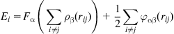
The EAM potential is a many-body potential function. The necessity of employing such a potential in nanoscale cutting simulations emerges from the fact that previous, simpler potential functions fail to account for the physics of metallic bonding. In fact, EAM-type potentials are now the most frequently used in simulations of metallic or alloy systems. This potential calculates the potential energy of the system as a combination of pair terms and an embedding function that is employed to determine the local energy density. This formulation considers the energy of the system as a function of electron density, where the density is assumed to be a superposition of the local atomic densities. Usually, an EAM potential is constructed by means of three functions: the aforementioned embedding function, an electronic density function, and a function that models potential due to pair exchange. The equation:

$E_i=F_{\mathrm{\alpha }}\left(\sum _{i\ne j}{\rho }_{\mathrm{\beta }}(r_{\mathit{ij}})\right)+\frac{1}{2}\sum _{i\ne j}{\phi }_{\mathrm{\alpha }\mathrm{\beta }}(r_{\mathit{ij}})$ (1.20)

(1.20)

where φ_αβ is a suitable pairwise potential function, ρ_β the contribution to the electron charge density from atom j of type β at the location of atom i, and F is a function representing the energy required to place atom i of type α into the electron cloud.

1.3.3 Boundary conditions and input parameters

As in the case of most types of simulation, boundary conditions are essential for the completion of the definition of a problem after the governing equations are properly derived. In the case of atomistic simulations, three types of boundary conditions exist in most cases: fixed boundary, thermal boundary, and periodic boundary conditions.

Fixed boundary conditions, one of the most common boundary condition in MD simulations of nanoscale cutting, resembles the fixed support in continuum mechanics problems or the behavior of a perfect rigid body (Shimizu, Eda, Zhou, & Okabe, 2008). In fact, these boundary conditions are implemented by keeping several layers at the sides of the workpiece fixed in their initial lattice positions throughout the simulation, as if these atoms were not affected by the process (Cheng, Luo, Ward, & Holt, 2003). This boundary condition provides a simple way to reduce some edge or more generally, boundary effects, and it helps to maintain the symmetry of the lattice (Goel, Luo, & Reuben, 2013; Yan, Sun, Dong, Luo, & Liang, 2006); although the workpiece dimensions also need to be large enough to reduce the impact of the fixed boundaries on the simulation results. These considerations can become essential to prevent an undesired rigid body motion caused by the interaction with other bodies, such as the cutting tool (Liang, Wang, Chen, Chen, & Tong, 2011; Rentsch & Brinksmeier, 2005; Zhang & Tanaka, 1997).

Thermal boundary conditions are also essential to almost every MD simulation of nanocutting. As the majority of cases is assumed to be conducted at vacuum conditions (Shimizu et al., 2008), there is no heat exchange between the workpiece and its environment. However, thermal effects within the workpiece are considerable. Specifically, during the nanocutting process, a significant amount of energy is converted into heat. To avoid artificial over-heating and temperature rise due to the finite volume modelled, the heat needs to be properly dissipated from the system to prevent affecting simulation results. Thus, it is important to define a suitable boundary condition that can act as a heat sink and also control the temperature of the workpiece.

In conventional machining, it is considered that a significant portion of cutting heat produced as a result of shear and friction energy can be carried away by lubricant or chip (Cheng et al., 2003; Goel, Luo, & Reuben, 2011). It is also shown (Narulkar, Bukkapatnam, Raff, & Komanduri, 2009) that from the heat attributed to plastic deformation of the workpiece, 10% is dissipated to the tool, 10% is dissipated to the workpiece, and almost 80% is carried away by the chip. Since most nanometric models are smaller than the systems they simulate, for reasons of computational cost, they are also not capable of sufficiently dissipating the produced heat within the modelled body (Goel et al., 2013; Narulkar et al., 2009). Therefore, layers of thermostat atoms are defined within the workpiece as a temperature-controlling layer (Cai, Li, & Rahman, 2007; Huang, 2013), usually between the fixed boundary layers of atoms and the surrounding, freely moving so-called Newtonian atoms, as seen in Fig. 1.6.

Newtonian atoms constitute the main, deformable region of the workpiece that interacts actively with the cutting tool or an energy source. This region forms a free boundary or is surrounded by layers of thermostat and fixed boundary atoms (Tong et al., 2014). The motion of the atoms within this region is computed from the direct numerical integration of Newton’s second law, according to the interatomic forces calculated from the potential function using a suitable and efficient algorithm to determine the list of atoms that interact with each other (e.g., neighbor-list) (Cai et al., 2007; Cheng et al., 2003; Goel et al., 2013; Oluwajobi & Chen, 2011b; Rentsch, 1996).

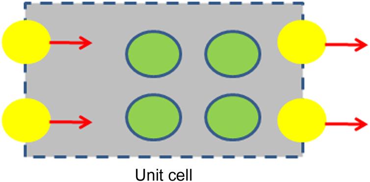
Another important type of boundary conditions are periodic boundary conditions. These involve taking a boundary particle—that has left the side where it belonged—and “returning” it to the opposite side of workpiece, in an effort to approximate a very large system, as it can be seen in Fig. 1.7. Relatively large systems in MD simulations serve to reduce boundary effects on simulation results (Cai et al., 2007; Rentsch & Brinksmeier, 2005). For these reasons, some researchers avoid using fixed boundary conditions, and periodic boundary conditions are often applied to the sides of workpiece along a specific direction (Goel et al., 2012; Hosseini, Vahdati, & Shokuhfar, 2011; Tanaka, Shimada, & Anthony, 2007; Yan et al., 2006; Ye, Biswas, Morris, Bastawros, & Chandra, 2003), or rarely, along two directions.

Although cutting speed can be considered a simple input parameter in most macroscopic machining simulations, it requires specific attention in nanoscale cutting simulations. As clearly seen in almost every work reported in the literature, most researchers consider the cutting speed employed, usually 20–200 m/s, to be significantly higher than the ones employed in real experiments; nanoscratching experiments are often used, usually in the range of 1–10 m/s (Gao et al., 2009; Ye et al., 2003). The latter are considered too slow to resemble realistic cutting conditions but can be employed for verification or calibration, with precaution and consideration of the experimental approach particularities. The primary reason for choosing a high cutting speed in modeling is that nanocutting simulations would either need extremely long time periods to complete or a considerable investment in computational infrastructure. Some investigations show clearly that there is an effect of speed on the results (Rentsch & Brinksmeier, 2005; Zhu, Qiu, Fang, Yuan, & Shen, 2014). However, in cases of high-speed cutting, in the range of 200–500 m/s, these large tool velocity values are acceptable and can be employed to simulate the processes in a realistic way.

1.3.4 Numerical integration and equilibration

The initial steps of modeling involves the determination of the workpiece and cutting tool geometry. Furthermore, process parameters, materials, and potential functions are chosen. Then starts the preliminary part of the calculation. The initialization of atom positions is first conducted during the geometry set-up, where atoms, assigned with an initial random velocity, are chosen relative to the temperature and other characteristics of the case and follow a Maxwell-Boltzmann distribution (Cheng et al., 2003; Goel et al., 2011; Maekawa & Itoh, 1995). After each atom’s initial velocities are assigned in the system and just before the simulation begins, it is also essential to relax the system for a specific period of time in order to adjust atom positions to close to equilibrium for a preset temperature. At that initial equilibration stage, the total energy is not conserved and potential energy can be transformed into kinetic energy and vice-versa by altering velocities and positions of atoms that move around their initial lattice positions until temperature fluctuations have ceased (Guo et al., 2010; Goel et al., 2011). It is strongly advised that atom trajectories at that stage should not be included in any kind of calculations. When the equilibration process has been completed, the total energy is preserved by means of the thermostat layer (Cai et al., 2007; Goel et al., 2011; Luo, Tong, & Liang, 2014; Tong et al., 2014), where a suitable velocity reset method is applied after a certain number of steps (Cai et al., 2007; Narulkar et al., 2009; Oluwajobi & Chen, 2011b; Yan et al., 2006), or when the temperature exceeds the predefined bulk temperature by five to ten K (Guo et al., 2010; Hosseini et al., 2011; Ye et al., 2003).

The numerical integration scheme is an important aspect of an MD simulation. Numerical solution of Newtonian equations requires a time-dependent integration method. For this reason, a variety of methods can be used, as in nonatomistic simulations. However, it is crucial to consider that not all integration schemes are effective in atomistic simulations, as a method that would require calculations of interatomic forces multiple times per timestep—like the Runge-Kutta family of methods, often suitable for many time-dependent simulations—contributes to a significant increase of computational time. Consequently, the most frequently employed integration methods are Verlet-type schemes and in some cases, predictor–corrector schemes.

Verlet method is the most widely used integration algorithm, often directly associated with MD simulations and specifically with the integration of Newtonian equations of motion. This algorithm is shown to exhibit good numerical stability, while having no significant cost than simpler methods such as Euler method. Verlet method is very popular in atomistic simulations, as it requires only a single calculation of forces per time-step, which is something already mentioned as very significant for this type of simulation. One formulation of Verlet algorithm (Störmer-Verlet formulation) is:

${\overrightarrow{x}}_1={\overrightarrow{x}}_0+{\overrightarrow{v}}_0\mathrm{\Delta }t+\frac{1}{2}{\overrightarrow{a}}_0{\mathrm{\Delta }t}^2$ (1.21)

(1.21)

${\overrightarrow{x}}_{\mathrm{n}+1}=2{\overrightarrow{x}}_{\mathrm{n}}-{\overrightarrow{x}}_{\mathrm{n}-1}+{\overrightarrow{a}}_{\mathrm{n}}{\mathrm{\Delta }t}^2,n=1,2..N$ (1.22)

(1.22)

where ${\overrightarrow{x}}_i$ represents the position vectors of system atoms at the time-step indicated by subscript i (ranging from 0 to N), ${\overrightarrow{v}}_i$ represents the velocity vectors of system atoms, ${\overrightarrow{a}}_i$ represents the acceleration vector at time-step n (equal to interatomic force vector ${\overrightarrow{F}}_i$ if all quantities are divided by atomic mass), Δt is the integration time-step, and N is the number of total time-steps in the simulation.

Furthermore, the Leapfrog scheme is a similar second order integrating scheme involving the calculations per time-step:

${\overrightarrow{x}}_{\mathrm{n}}={\overrightarrow{x}}_{\mathrm{n}-1}+{\overrightarrow{v}}_{i-1/2}\mathrm{\Delta }t$ (1.23)

(1.23)

${\overrightarrow{a}}_{\mathrm{n}}=F({\overrightarrow{x}}_{\mathrm{n}})$ (1.24)

(1.24)

${\overrightarrow{v}}_{\mathrm{n}+1/2}={\overrightarrow{v}}_{\mathrm{n}-1/2}+{\overrightarrow{a}}_{\mathrm{n}}\mathrm{\Delta }t$ (1.25)

(1.25)

Predictor–corrector integration schemes are numerical integration schemes with a more complex formulation and consist of two major steps: a prediction step where a simpler integration method is used to provide a first approximation of the result and then a more robust method is applied to “correct” this result. This is usually accomplished by using a suitable combination of an explicit and an implicit method, for prediction and correction purposes, respectively, so as the process converges effectively.

Finally, it should be noted that various limitations and particularities render MD simulation computationally demanding, even for relatively moderate atomistic systems. It is worth noting that multiscale models, involving FEM and MD combination analysis can be found in the literature (Pen, Bai, Liang, & Chen, 2009). This approach exploits the capabilities of continuum and micromechanics models and simultaneously reduces the computation cost of a full atomistic simulation. More effective algorithms and state-of-the-art computational systems capabilities need to be taken seriously when novel and demanding studies with greater and more realistic models and fewer assumptions are employed.