Creating an Office PivotTable List

An Office PivotTable list is superficially similar to an Excel PivotTable report. Both tools can link to an Analysis Services cube. Both tools can use a member to filter, and both tools allow you to show and hide levels of a dimension on an axis. But the tools behave differently in many ways. With an Excel PivotTable report, the ability to communicate with an OLAP cube was added to an existing feature, and the user interface sometimes seems more closely adapted to the old features than to the new ones. The interface for an Office PivotTable list was created with OLAP cubes in mind, so the PivotTable list is often a more flexible tool for working with an OLAP cube.

Create a PivotTable List from a PivotTable Report

The easiest way to add a PivotTable list to a Web page is to first create a PivotTable report in Excel and then publish the PivotTable report as an interactive Web page.

1.	Activate the Chart Report sheet of the Chapter 5 workbook. On the File menu, click Save As Web Page. [View full size image]
2.	In the Save As dialog box, click the Publish button.
3.	Under Item To Publish, select PivotTable in the list. Under Viewing Options, select the Add Interactivity With check box and select PivotTable Functionality from the drop-down list. Select the Open Published Web Page In Browser check box, and click Publish. Your browser must be able to use ActiveX controls for you to browse the PivotTable list. The Office PivotTable list appears in the browser window. An Excel PivotTable report toolbar automatically shows each dimension and measure as a button when part of the report is selected. The Office PivotTable list toolbar contains a single button that displays a list of dimensions, levels, and measures. [View full size image]
4.	On the toolbar, click the Field List button. The PivotTable Field List window appears. This field list is roughly equivalent to the list of buttons on an Excel PivotTable toolbar. Tip The PivotTable list report created from an Excel workbook is always centered within the browser window, making it difficult to position the PivotTable field list in the margin. If you resize the browser window to take up only a portion of the screen, the PivotTable list will center itself within the smaller browser window and you can position the field list outside the browser window.
5.	Click the PivotTable list heading. Then, on the toolbar, click the Property Toolbox button. The PivotTable Property Toolbox appears. This toolbox includes properties appropriate to the currently selected portion of the PivotTable list.
6.	Click various places on the PivotTable list to watch the contents of the PivotTable Property Toolbox change. An Excel PivotTable has no direct equivalent to the property toolbox.

Manipulate Levels in a PivotTable List

In an Excel PivotTable report, you interact frequently with dimensions and members but not with levels. Dimension levels appear and disappear as you show or hide detail for members on the report, and the button for the top level is the only one that ever displays a drop-down list. In an Office PivotTable list, you can deal much more directly with levels within a dimension.

1.	In the PivotTable list, expand the Bread member. The children of Bread appear under the Subcategory level heading. None of the subcategory labels shows a plus sign, however, even though the Product dimension contains one more level of detail below Subcategory. If you try to double-click the Bagels member, nothing happens. [View full size image]
2.	In the PivotTable Field List window, expand the Product dimension. Select the Product Name level. Then, at the bottom of the field list window, in the Add To drop-down list, select Row Area and click Add To. The Product field appears in the PivotTable list. [View full size image] You can also drag the Product level to the row area of the PivotTable list.
3.	Expand the Bread member, and then expand the Bagels member. [View full size image] In an Excel PivotTable report, a level appears on an axis only if members from that level are visible. Showing the children for a member adds the next level if it’s available. In an Office PivotTable list, levels can be added to or removed from an axis, even if no members are visible. You can see only members from levels that are explicitly on an axis. Note The use of levels in a PivotTable list also affects what you see in the dimension tree. In an Excel PivotTable report, selecting or deselecting items in the dimension tree determines whether that item will appear on the axis, and levels are added if necessary. In an Office PivotTable list, selecting or deselecting items in the dimension tree merely filters those items. In other words, deselecting an item hides it in the dimension tree, but only if that item would otherwise be displayed.
4.	Drag the Subcategory level label past the edge of the PivotTable list. (A red X appears on the mouse pointer.) This removes the Subcategory level, leaving only the Category level and the Product Name level on the row axis. [View full size image]
5.	Expand the Bread and Dairy members. All the Products in the Bread category appear; they just aren’t grouped by the Subcategory level members. [View full size image]
6.	Drag the Category label off the PivotTable list. The report shows the complete list of products, still arranged in the order of the category and subcategory groups. This is the hierarchy order for the members, and it’s the default order for members of a level even if the parent members aren’t visible. You can override the default sort order. [View full size image]
7.	Click the Product Name level label, and activate the PivotTable Property Toolbox. Expand the Sort section of the toolbox, and select Ascending from the Sort Direction drop-down list. [View full size image] You can also sort the list of products in descending order of total sales. Unfortunately, you cannot use the PivotTable Property Toolbox to do this.
8.	Right-click any cell in the Grand Total column, and click Sort Descending from the shortcut menu. The list of products sorts in descending order. [View full size image] Sorting by a measure column removes the sort direction from the row members or from any other measure column.
9.	Select the Sort Descending command a second time to remove the Sort Descending flag for the measure. This sets the sort for the Products back to the default, not to the sort direction set previously. [View full size image]

In an Excel PivotTable report, you can not have a report that shows all products at only the Product level—sorted or not. An Office PivotTable list gives you more control over how to use levels within a report.

Manipulate Subtotals in a PivotTable List

An Excel PivotTable report always shows the complete subtotal for a group, even if some of the items are hidden. An Office PivotTable report allows you more control over how to display subtotals.

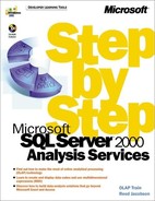
1.	Click the Time dimension drop-down arrow, select the 1998 check box, and click OK. [View full size image] The total in the Sales Units column for Bagels in 1998 was 984. This is equal to the sum of sales units for the three countries. Hiding the USA column demonstrates how the PivotTable list manages totals.
2.	Click the Country drop-down arrow, clear the USA check box, and click OK. The total for Bagels is still 984, even though that total doesn’t equal the sum of the two visible countries. An asterisk follows the Grand Total label. The asterisk indicates that the total might include hidden items. [View full size image]
3.	Click the PivotTable list caption bar (to select the entire PivotTable list). Activate the PivotTable Property Toolbox, and expand the Totals section. Clear the Total All Items check box. The value in the Grand Total column changes to 232, which is the sum of the two visible countries. The asterisk also disappears from the Grand Total label. [View full size image] Note In an Excel PivotTable report, subtotal labels include a trailing asterisk as a default. In the PivotTable Options dialog box, you can turn off the trailing asterisk. In an Excel PivotTable report, however, you can’t make the subtotals match the total of only the visible cells.
4.	Click the Country label drop-down arrow, select the Show All check box, and click OK to redisplay USA. The total changes to match the sum of the visible cells. Your hypothetical company didn’t start selling products in Mexico until the third quarter of 1998. You can choose how Mexico totals are displayed when no data is available.
5.	Click the Time drop-down arrow, expand 1998, select the Quarter 1 check box, and click OK. Mexico disappears from the list of countries. [View full size image]
6.	With the entire PivotTable list selected, activate the PivotTable Property Toolbox and expand the Display Empty Items section. Select the Column check box. The Mexico member reappears, even though all the cells for the column are blank. [View full size image]
7.	Clear the Column check box for Display Empty Items. Then Drag the Sales Dollars measure from the Field List window to the data area, to the right of any Sales Units column. The new measure appears in the Columns area. Unlike an Excel PivotTable report, where multiple measures create a new Data dimension, an Office PivotTable list has a property for controlling the orientation of the measures. [View full size image]
8.	With the entire PivotTable list selected, activate the PivotTable Property Toolbox and expand the Totals section. In the Total Orientation dropdown list, select Row. The two measures switch to the row axis. [View full size image]
9.	Close the browser.

A PivotTable list gives you a great deal of flexibility in how to deal with measures—or totals, as they’re called in the PivotTable list.

Design a PivotTable List in FrontPage

You use a browser such as Microsoft Internet Explorer to display a PivotTable list. Within the browser, you can rearrange dimensions and change formatting. When you close the browser, however, all changes you made are lost. The next time you open the page containing the PivotTable list, the list returns to its original state. To create or define a PivotTable list, you must use an application capable of entering design mode. FrontPage, included in the Premium edition of Office 2000, is capable of designing a PivotTable list.

1.	Start FrontPage. With a blank, new page active, on the Insert menu, point to Component and click Office PivotTable. An empty PivotTable list, showing the text No Data Source Specified, appears. Your first task is to define a data source.
2.	On the PivotTable list toolbar, click the Property Toolbox button (one of the few buttons that’s not disabled). In the PivotTable Property Toolbox, expand the Data Source section.
3.	Under Get To Data Using, click the Connection option and click the Connection Editor button. This dialog box is similar to the Data Link Properties dialog box used in Analysis Manager, except this one defaults to use Microsoft SQL Server as a provider.
4.	Click the Provider tab, and select Microsoft OLE DB Provider For OLAP Services 8.0.
5.	Click Next, and type localhost or the name of the computer running the Analysis server in the Data Source box. In the Enter The Initial Catalog To Use drop-down list, select the Chapter 5 database. Then click OK. You still need to specify a cube from the database.
6.	Under Use Data From in the PivotTable Property Toolbox, click the Data Member option and then select Sales from the drop-down list. The PivotTable list immediately changes to show the drop areas. [View full size image]
7.	Click the Field List toolbar button. Drag Sales Units to the Totals area, drag Product to the Filter area, drag Time to the Column area, and drag State to the row area. [View full size image]
8.	Click the Preview tab to see how the control will appear in a browser. Click the Save button, type Market Test as the name of the HTML file, and click Save. Any changes you make to the document while in FrontPage—whether on the Normal tab, the HTML tab, or the Preview tab—will be retained in the HTML file.

When you want control over the initial layout of a PivotTable list, you need to use a design program to make the changes. An HTML editor such as FrontPage can serve as a design program for the Office PivotTable list.

Create a Restricted PivotTable List

You might want to create a PivotTable list for others to use. Often, you want to provide some of the functionality of the PivotTable list but not all. For example, you might want to allow users of the list to drill down from a member to its children on the row axis but not move dimensions from one axis to another, change filters, or change formatting. With an Excel PivotTable report, you can write Visual Basic macros to restrict the capabilities of the report, but by using an Office PivotTable list, you can restrict the capabilities without any programming.

1.	In FrontPage, click the Normal tab to change to design mode for the PivotTable list. Customize certain settings before restricting the capabilities of the PivotTable list.
2.	In the Product drop-down list, select the Bread check box, and click OK. In the Country drop-down list, clear the check boxes for Mexico and Canada, leaving only USA selected, and then click OK. Select the Country caption, and click the Subtotal button in the toolbar to remove the redundant Grand Total row. Drag the Quarter level label from the report, leaving only Year and Month. This is the general structure of the report you’ll allow users to see. [View full size image]
3.	Click the caption bar of the list (to select the entire list), and click the Property Toolbox toolbar button. Expand the Advanced section. The PivotTable Property Toolbox contains sections in design mode that aren’t available when viewing the list in a browser.
4.	Clear the Allow Property Toolbox check box. This prevents a user from changing the formatting of the PivotTable list. Select the Lock Filters check box and the Lock Row/Column Fields check box. This prevents a user from moving dimensions from one area to another or displaying items you have filtered.
5.	In the Maximum Height box, type 480. In the Maximum Width box, type 640. This keeps the PivotTable list from expanding beyond the specified size. If the PivotTable list becomes larger than these dimensions, it will display scroll bars.
6.	Collapse the Advanced section of the toolbox, and expand the Show/ Hide section. Click the Toolbar button to hide the toolbar from the PivotTable list.
7.	Save the HTML page, and click the Preview tab to see how the PivotTable list will appear to a user. Try expanding and collapsing members. Notice the horizontal scroll bar that appears when you expand years. Try dragging level labels off the list or to a different area. Try displaying values for Meat, Dairy, Mexico, or Canada.
8.	Close FrontPage.

As a PivotTable list designer, you can limit the capabilities you allow a user. By using an Office PivotTable list, you can generate a list that provides considerable flexibility—particularly for drilling down to detail levels—without writing any customization code.