Understanding OLAP Processing

In this section, you’ll learn what happens when you process an Analysis Services database. This includes looking at how the Analysis server processes a dimension as well as how the server processes a cube. You’ll learn what happens to client applications while the server is processing a database, and you’ll learn what happens when the data warehouse changes and you haven’t processed the OLAP database.

How the Analysis Server Processes a Dimension

When you process a dimension, the Analysis server creates a SQL statement to extract the necessary information from the data warehouse dimension table. The extract includes one or two columns for each level in the hierarchy. (If the Member Name Column property for a level is the same as that of the Member Key Column, the Analysis server extracts only the key column. If the name column is different, the Analysis server extracts both.) The Analysis server retrieves one row from the data warehouse for each distinct combination of level keys and sorts the rows using the Member Key Column property of each level. As an example, say you want to process the State dimension in the Chapter 9 sample database. To generate the State dimension from the Chapter9 warehouse, the Analysis server extracts the following rows:

The State level has both a STATE_ID and a State_Name column; the Region and Country levels have one column each. The rows are sorted first by Country, then by Region, and finally by State_ID. The retrieved rows represent, if you will, the dimension members from the warehouse perspective. The structure of the relational columns does not show that the members of the Region level are children of the State level. The Analysis server needs to create the dimension members from the hierarchy perspective. For each member of the dimension, the server creates a unique path that contains a component number for each level in the dimension. The State dimension contains three levels, so the path for each member will contain three numbers, one for each level: Country→Region→State.

Starting with the first row retrieved from the relational table, the server creates a new member for each relevant level of the hierarchy. So, for the row containing information about British Columbia, the server starts by creating a member with the path 0→0→0, which corresponds to the All level member of the dimension. (In the Chapter 9 OLAP database, the name of the All level member is North America.) The server then creates a member with the path 1→0→0, which corresponds to the Canada country. The server then creates a member with the path 1→1→0, which corresponds to the Canada West region. Finally the server creates a member with the path 1→1→1, which corresponds to the British Columbia state. The server created four members based on the first row from the relational dimension. For the second row, the server creates only three members, since the All level member already exists. By the time the server has finished, it has created a unique path for each member of the dimension. That path contains the genealogy of each member. For the State dimension, the server creates the member names and paths shown in the first two columns of the following table:

To create the path, the server always sorts the children of a member by using the value from the Member Key Column property, regardless of the value in the Order By property for a level. After creating the paths, the server creates a separate ID for each member that does take into consideration the Order By property, sorting by member name as a default. In the preceding table of the State dimension members, the third column shows the ID for each member. In the State dimension, the sequence of the ID numbers matches the sequence of the path numbers, except for Oregon and Washington. The path sequence puts Washington before Oregon because the STATE_ID for Washington (1) precedes the STATE_ID for Oregon (2). The ID sequence puts Oregon before Washington because the State_Name for Oregon alphabetically precedes the State_Name for Washington. The ID numbers sort members into what is called the hierarchy order. The hierarchy order is the order for the members if a multidimensional expressions (MDX) query retrieves all the members the dimension.

As mentioned earlier, the path for each member contains the member’s complete genealogy. The Analysis server combines the paths from all the members to create a map for the dimension. The dimension map allows the Analysis server to slice and dice hierarchies very quickly. You don’t need to remember (or even really understand) exactly how the Analysis server creates a map for each dimension, but understanding that the family tree is built into each member can help you understand certain behaviors and rules that otherwise might seem arbitrary.

How the Analysis Server Processes a Cube

As explained in Chapter 8, “Storage Optimization,” many OLAP products have a problem with data explosion—creating massively large cube files from even moderately large warehouse data. Analysis Services, however, is remarkably efficient in the way it stores data in a cube, often creating a cube that is much smaller than the original data source. The actual physical structure of Analysis Services cube files is proprietary to Microsoft, and understanding it perfectly would not be helpful. But creating a meaningful conceptual picture of a cube can help you both as you design a cube and as you retrieve reports from it.

As you learned in earlier chapters, a cube consists of one or more dimensions combined with one or more measures. Those dimensions form the structure or organization for the data values in the cube. Before the Analysis server can process a cube, it must have already processed each dimension used in the cube.

When you process a cube, the Analysis server executes a SQL statement to retrieve values from the fact table. The SQL statement retrieves enough columns to completely identify each member and the columns for the measures. For each row extracted from the fact table, the Analysis server identifies for each dimension the member that corresponds to that row. It then creates a compound path for the row. For example, the following table contains the first four sample rows extracted to create the first cube in the Chapter 9 OLAP database:

Each row includes two dimensions: Year and State. The server finds the leaf-level member path for each dimension. For the first row, the path for Year 1997, Quarter 1, Month 1 is 1→1→1. As mentioned in the preceding section, the path for the Washington state is 3→1→1. From these two paths, the Analysis server constructs a single path for this combination of members, which you can picture schematically as 1→1→1·3→1→1. This is the internal path for one cell of the cube: Washington in January 1997. In other words, the path for a cell in a cube is an internally generated number consisting of one subnumber for each level for each dimension used in the cube. The cubes in the Chapter 9 database contain two dimensions (Time and State), both of which have three levels (not counting the All level). That means that each cell in the Sales cube has a path consisting of 6 numbers—one for each of the three levels in each of the two dimensions. The Sales cube in the FoodMart 2000 sample database has 10 dimensions actually stored in the cube, with a total of 23 levels between the 10 dimensions. (In Foodmart 2000, the Store Size In SQFT and Store Type dimensions are virtual dimensions, which are not stored in a cube. Virtual dimensions are explained in Chapter 10, “Dimension Optimization.”) That means that each cell in the FoodMart 2000 Sales cube has a path consisting of 23 numbers. The more dimensions a cube has—and the more levels in each dimension—the more information is stored in each cell of the cube.

When the Analysis server begins processing a cube, it creates a data file to store the cells for the cube. When the server processes a single row extracted from the fact table, it first calculates the path for the leaf-level cell. From the previous table, the path for the first row of sample data looks like this:

1→1→1·3→1→1 (1997→Quarter 1→January·USA→North West→Washington)

The server checks to see whether a leaf-level cell with that path already exists. If the cell exists, the server adds the new measure to the one already in the cell. If the cell does not already exist, the server creates a new leaf-level cell, storing both the path and the value of the measure. (The leaf level isn’t created if you choose HOLAP or ROLAP storage mode when you design storage for your cube.)

After creating a leaf-level cell, the Analysis server creates cells for any aggregations you designed. Now assume that the cube had three aggregations designed: Quarter by North America, Year by Region, and All Time by State Code. The Analysis server simply creates the appropriate three subsets of the original cell path:

1→1→0·0→0→0 (1997→Quarter 1·North America)

1→0→0·3→1→0 (1997·USA→North West)

0→0→0·3→1→1 (All Time→·USA→North West→Washington)

Each of these paths corresponds to the path of an aggregated cell. If the cell already exists, the server adds the measure value to it; if the cell doesn’t exist, the server creates the cell and stores the measure value. That then completes the processing for one row.

The server repeats this process for each row extracted from the fact table. Because the path for a cell contains the complete genealogy for the member of each dimension in the cell, calculating the path for each aggregate value is relatively straightforward. Along with creating the data file, Analysis Manager creates various index files to facilitate rapid retrieval of the values. Once all the values have been accumulated, the Process log window in Analysis Manager announces that processing has completed successfully.

Watch the Server Process a Database

The Analysis server uses the concept of a transaction when processing a database. When the server begins processing the database, it begins a new transaction. When it completes processing, it commits the transaction. If, for some reason, processing isn’t completed successfully, the server rolls back the transaction and the database looks like it did before the transaction started. During the course of the transaction, all changes are made to temporary files so that applications retrieving values from the server are not aware that a transaction is taking place.

When you process a database, all the dimensions and all the cubes are processed within a single transaction. This means that all users can continue to use any cube or dimension with the database—seeing no changes—until the entire database has processed. Also, if anything should go wrong during the processing, all the temporary files are deleted—or rolled back—and the database remains as if nothing had happened. You can watch the server create and rename temporary files by looking at the data folder while processing the database.

1.	In Windows Explorer, open the Chapter 9 folder within the OLAP Data folder. (You specify the location of the OLAP Data folder when you install Analysis Services. By default, this folder is under Program FilesMicrosoft Analysis ServicesData on the Windows drive.) You should see four files for each dimension and one file for each cube within the database, plus a folder for each cube and a few other files.
2.	On the View menu, select Details. Make a note of the date and time each file was last modified. (You might want to tile the Analysis Manager and Windows Explorer windows vertically so you can see both at the same time.) [View full size image]
3.	Switch back to Analysis Manager, right-click the Chapter 9 database, and click Process The Database.
4.	As soon as the Process log window opens, switch to the Windows Explorer window that displays the database files. Press the F5 function key to refresh the window. You’ll see new files and folders appear, each with extra characters included in the name. [View full size image] As soon as the database completes processing, you’ll see the temporary files disappear and you again see single names for the files in the database. The date and time for these files, however, does indicate that they’re the new versions of the files. [View full size image]
5.	In Analysis Manager, close the Process log window.

You might wonder what happens to a client application that’s browsing a cube in the database at the time the database is finished processing, particularly as the client has its own cache and can retrieve some values from that cache while requesting only needed new values from the server. The Analysis Services client component, PivotTable Service, sends a request to the server every 10 seconds asking the server whether the active database has changed. Once the database has completed processing, the server communicates the change to the PivotTable Service, which erases all the old values from the client cache.

Changing Data in a Warehouse

When you process an OLAP database, you make information in the cube and dimensions match the information stored in the data warehouse, using the rules, or schema, you created when you designed the database. If you change the schema—for example, if you add a measure or a dimension to a cube—you must process at least the affected portions of the database. You also need to process at least a portion of the database if the information in the data warehouse changes, as it inevitably will.

The information in a data warehouse is almost always time dependent. That means that, at the very least, you’ll continually add new time periods to your data warehouse. In time, you might also add additional products or additional sales regions. When the data warehouse changes, you need to process the database to resynchronize the OLAP database with the relational data warehouse.

The SalesFact table in the Chapter9 sample Microsoft Access database contains data for six geographical areas (states) through October 1998. In the Chapter9 database, the State dimension table includes only the six states that appear in the fact table. The TimeMonth dimension table, however, includes months through December 1998. It is not uncommon in a warehouse to include months in the time dimension through the end of the current year, but to add members to other dimensions only as they are needed.

Included in the same folder as the Chapter9 database is a database named Chapter9a. The Chapter9a database schema is identical to that of the Chapter9 database, and the Chapter9a database includes all the data in the Chapter9 database. It also includes some additions: one new entry in the State table (Vera Cruz, Mexico) and additional rows in the fact table for a new month (November 1998). Switching the data source for the Chapter 9 OLAP database from Chapter9 to Chapter9a simulates adding new values to the data warehouse.

Set Storage Options for Sample Cubes

The Chapter 9 database contains seven identical cubes. For each of these cubes, the storage option is set to the default MOLAP with no aggregations. Before changing the data source, assign different types of data storage to two of the cubes, to see the effect that changing the data source has, using different data storage methods.

1.	In the Cubes folder of the Chapter 9 database, right-click the Sales2 HOLAP Detail cube, and click Design Storage. Click Next to skip the welcome screen.
2.	Select the HOLAP storage mode, and click Next.
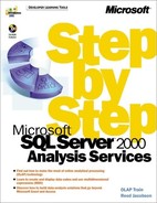
3.	Click the Until I Click Stop option, and click Next. This creates a HOLAP cube with no aggregates. [View full size image]
4.	Leave the Process Now option selected, and click Finish. Close the Process log window. Processing with HOLAP storage and no aggregations takes virtually no time because the server doesn’t need to even read the fact table.
5.	Right-click the Sales3 HOLAP Aggregated cube, and click Design Storage. Click Next to skip the welcome screen.
6.	Select the HOLAP storage mode, and click Next.
7.	Click the Performance Gain Reaches option, and leave the percentage at 50.
8.	Click the Start button, wait until the Next button becomes enabled, and click Next. The wizard designed three aggregations. [View full size image]
9.	Leave the Process Now option selected, and click Finish. Close the Process log window. With HOLAP storage, if you design aggregations, the server creates cells in the data file for aggregations.

You now have the Sales1 MOLAP cube with MOLAP storage and no aggregations, the Sales2 HOLAP Detail cube with HOLAP storage and no aggregations, and the Sales3 HOLAP Aggegated cube with HOLAP storage and three aggregations.

Browse Data Before Updating the Warehouse

In this section, you’ll look at the values in the cubes before you change the data source. Each cube has identical contents, but you can arbitrarily browse the Sales MOLAP cube as an example. You can check for key values from that one cube.

Change the Database Data Source

Because the internal objects within the database refer only to the data source, you can change the definition of the data source without disrupting the database, as long as you don’t change the internal structure of the data source. When you edit a data source, you get the same Data Link Properties dialog box as when you create a data source but with a different tab active initially.

1.	In the Analysis Manager console tree, expand the Data Sources folder in the Chapter 9 database.
2.	Right-click the Market data source, and click Edit.
3.	Adjacent to the Select Or Enter A Database Name box, click the ellipsis (...) button, select the Chapter9a database, and click Open. [View full size image]
4.	Click OK to close the Data Link Properties dialog box.

The name of the data source doesn’t change; only the definition changes. By clicking the Provider tab, you could change the data source from an Access database to a Microsoft SQL Server database, for example, or from an OLE DB data source to an ODBC data source. The OLAP database will work the same, as long as the relational database schema remains unchanged.

Browse Data After Updating the Warehouse

Now that you have effectively changed the data in the data warehouse, the cubes in the OLAP database no longer match the data in the warehouse. The way a cube behaves depends on the storage mode of the cube. To see what values changed, start by browsing the data in the Sales1 MOLAP cube.

1.	Select the Sales1 MOLAP cube, and click the Data tab at the top of the right pane to browse the cube. Expand the Mexico and Mexico Central members to see the states. The grand total is 35,696, and Vera Cruz doesn’t appear in the list of states. All these values are unchanged from before the warehouse changed. [View full size image] The Sales MOLAP cube uses MOLAP storage, and it behaves as if you had not changed the data source. When you use MOLAP storage, with or without aggregates, the cube is completely detached from the data warehouse. You can even delete the warehouse database without affecting the OLAP database.
2.	Select the Sales2 HOLAP Detail cube, and browse it in the Data pane. In this cube, the Sales Units total is 42,243, which is different from the previous 35,696 total. Because there are no aggregations designed for the cube, all the values are aggregated from the relational data store immediately. Problems arise, however, when you attempt to browse to an area where new members exist in the fact table that aren’t represented in the dimension.
3.	Double-click the Country level button to display the Region level. The Region list for Mexico still shows only Mexico Central—Mexico West has not yet been added to the dimension—but the values change to show #ERR. The server has recognized a discrepancy in the dimension hierarchy.
4.	Select the Sales3 HOLAP Aggregated cube, and browse it in the Data pane. This Unit Sales total is 35,696, unchanged from the original warehouse, as if this were a MOLAP cube. [View full size image] Even though this cube uses HOLAP storage mode and uses the relational data source for the leaf level values, some aggregates are physically stored in the cube file.
5.	Drag Time to the row area (replacing the State dimension), and expand the 1998 and Qtr4 members. The total for Nov is 6,547, the new value. This value came from the fact table. [View full size image] The total for Qtr4, however, is still 4,545, the prestored aggregated value. Clearly, 4,545 is not the sum of 4,545 and 6,547. The quarter value doesn’t match the sum of the month values. In HOLAP mode (and ROLAP is the same), some cell values are generated from the fact table and use the new values, while other cell values are generated from aggregated values and use the old values.

Cubes that use HOLAP or ROLAP data storage and include at least one aggregation retrieve some cell values directly from the relational source and other cell values from the stored aggregations. This fact makes HOLAP and ROLAP storage modes vulnerable to inconsistencies in cell values. You should always process databases containing HOLAP or ROLAP cubes as soon as the data warehouse changes. In MOLAP storage mode, all cell values—detail and aggregated alike—are oblivious to the data warehouse unless you explicitly process the database. You can even delete the data warehouse without affecting the cube.