Specifying Options for Optimizing Storage

The reason to add an OLAP layer to a data warehouse is to make data retrieval flexible and fast. As you learned in Chapter 1, the cube structure, with a hierarchy defined in each dimension, makes interacting with the cube flexible because you can drill up and down the hierarchies and slice or dice by dimension members. To make the data retrievals fast, Analysis Services summarizes selected values and stores them as predefined aggregations. You define aggregations in a cube, by first specifying the appropriate storage modes for the cube.

Understand Analysis Server Storage Modes

As you learned in Chapter 2, an Analysis Services cube consists of three logical components: a map, detail values, and aggregated values. The map stores hierarchical information about the members of all dimensions used in the cube. The detail values correspond to the lowest-level members of each dimension. (If the cube has the same dimensions at the same level of detail as the fact table, the detail values in the cube match the values in the fact table.) The aggregated values are summarized values for higher levels in dimension hierarchies.

An OLAP cube always stores the cube map within the Analysis server, but Analysis Services allows you to decide where to store the detail and aggregated values. You can choose from three physical storage options: ROLAP, HOLAP, and MOLAP.

• ROLAP, for relational OLAP, leaves detail values in the relational fact table and stores aggregated values in the relational database as well.

• HOLAP, for hybrid OLAP, leaves the detail values in the relational fact table but stores the aggregated values in the cube.

• MOLAP, for multidimensional OLAP, stores both detail and aggregated values within the cube.

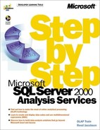
If you picture storage in a relational database as a cylinder and storage within Analysis Services as a cube, the three options appear as in the following graphic:

All three storage modes include the cube map within Analysis Services. It’s the cube map that makes the data appear as a cube to a person running a query. That means the storage mode is invisible to client applications—that is, applications that query the cube. The client application always sees the cube. The storage option you chose affects only performance.

Because a client application can’t tell which storage mode you have chosen, you can change the storage mode without affecting any client applications. Once you specify storage and start using the cube, you can change your mind later and switch to a different storage type. Because a cube appears to the client application as a single, logical entity, you can use different storage modes for different portions of a cube. In order to do that, you must use multiple partitions, which you’ll learn about in the section “Working with Partitions” in Chapter 9, “Processing Optimization.”

Choose the Correct Storage Mode

Choosing a storage mode is not as difficult as it might seem. In the first place, using Analysis Services to store aggregations in a relational database never makes any sense, so you should never choose the ROLAP option. Aggregations in a relational database are both bulky and slow. The purpose of creating aggregations is to improve performance, and relational aggregations defeat the purpose. The only reason you might choose the ROLAP option is if you’re learning about aggregations and want to physically look at aggregations. The following section in this chapter uses ROLAP storage to help you understand aggregations. As you’ll see when you look at ROLAP aggregations, they’re completely unusable by any application other than Analysis Services.

Aggregations in both MOLAP and HOLAP are identical, so the only difference is where the detail-level values are stored. If you count the space required by the original warehouse as well as the space needed for the OLAP cubes, MOLAP does consume more storage space than HOLAP because the MOLAP storage option does duplicate the values from the fact table. Analysis Services, however, is efficient in how it stores data. For example, a freshly compacted Microsoft Access database containing only the SalesFact table from the Market database takes 588 KB of storage space. A cube containing the same level of detail (with no aggregations) takes only 78 KB of storage space! With a very large warehouse database, you could process the data into a MOLAP cube and then archive and remove the original warehouse. By using the MOLAP storage option, you could actually end up using a small fraction of the original storage space.

If you have a large, permanent warehouse, and if using aggregations can satisfy most queries, HOLAP storage is an excellent option. Queries that must go to the detail data will be slower than if the cube used MOLAP storage, but if they’re infrequent, the performance gain might not be worth the incremental storage requirements. In addition, processing a MOLAP cube can take more time than processing a HOLAP cube. While developing an OLAP cube—during the time that you might process frequently—you might want to use HOLAP storage simply to speed up processing. Once you have completed the database design, you can switch to MOLAP storage to maximize query performance.

Understand Analysis Server Aggregations

Aggregations are precalculated summaries of detailed data that enable the Analysis server to answer queries quickly. While you can easily create a cube without aggregations—none of the cubes used previously in this book have any aggregations—aggregations can make a tremendous difference in query time for a large cube. As with storage mode, aggregations are invisible to client applications. Regardless of how many aggregations you design, the cube always appears to contain every possible aggregated value. When you request a value from a cube, Analysis Services uses whatever aggregations are available to retrieve the value as quickly as possible.

You also don’t need to store all the possible aggregations for a cube. The Analysis server can use aggregations that do exist to quickly calculate additional values as needed. For example, say you request the total Sales Dollars for 1999 from a Sales cube and that aggregated value is not physically stored in the cube, but the quarter totals are. The Analysis server will retrieve the four quarter totals and quickly calculate the year total.

Don’t confuse an aggregated value with an aggregation. An aggregated value is a single, summary value retrieved from a cube. An aggregation consists of all the possible combinations of one level from each dimension in the cube. The easiest way to understand what aggregations are is to create some simple cubes—designing all the possible aggregations and using the ROLAP storage mode—and then look at the aggregation tables in the relational database.

Inspect Aggregations for a Single Dimension

The simplest possible cube contains a single dimension. Following the steps below, you can create a cube based on the Chapter 8 data warehouse that has only the Time dimension. You’ll use the Storage Design Wizard and choose the ROLAP storage option to create all the possible aggregations. Later in this chapter, you’ll learn how to use the Storage Design Wizard to refine the choice of aggregations.

1.	In Access, open the sample Chapter 8 database. Before creating ROLAP aggregations, the database contains only the fact table and dimension tables. [View full size image]
2.	Switch to Analysis Manager, and then expand the Chapter 8 database. Right-click the Cubes folder, point to New Cube, and click Wizard.
3.	Click Next to skip the welcome screen.
4.	Select SalesFact as the fact table, and click Next. Add Sales_Dollars and Sales_Units as the measures, and click Next. Add Time as the dimension, and click Next. Click Yes when cautioned about counting rows in the fact table. Type Time Only as the name of the cube, and click Finish.
5.	In the Cube Editor, on the Tools menu, click Design Storage. Click Next to skip the welcome screen. Select ROLAP as the data storage type, and click Next. [View full size image]
6.	When asked to set storage design options, click Start, wait until the Start button changes to Continue and the Next button becomes enabled, and then click the Next button. [View full size image]
7.	On the final screen of the wizard, leave the Process Now option selected and click Finish. If the wizard displays a warning about possible problems with creating ROLAP storage in the data source, click Yes to continue. After the cube finishes processing, close the Process log window.
8.	Switch to Access, and press F5 to refresh the Database window. You’ll see four newly created tables, each beginning with the prefix TimeOnly_ TimeOnly_, and ending with a number. Each table corresponds to a single aggregation. [View full size image]
9.	Open, inspect, and close each of the aggregation tables starting with TimeOnly_TimeOnly_4 and ending with TimeOnly_TimeOnly_1. TimeOnly_TimeOnly_4 contains columns for Year, Quarter, and Month, along with columns for the summarized measures—Sales Units and Sales Dollars; the table contains 22 rows, one for each member of the Month level of the Time dimension. [View full size image] TimeOnly_TimeOnly_3 contains, aside from the measures columns, columns only for Year and Quarter; the table contains 8 rows, one for each member of the Quarter level. TimeOnly_TimeOnly_2 contains only the Year column, aside from the measures, with two rows. TimeOnly_TimeOnly_1 contains only the summarized measure fields and has only a single row because this aggregation corresponds to the All level of the cube.

With a single dimension in the cube, each aggregation corresponds to a single level from the dimension. The following table shows the four levels in the dimension, with each label showing the number of members in the level. The second column shows the actual number of rows in the table over the theoretically possible number of rows for that level. (Because the Time dimension came from the fact table, the actual number is always the same as the theoretical number.) The suffix for each aggregation table is in brackets.

Fully aggregated, this cube has 33 aggregated values for each measure, but in the terminology of Analysis Services, it has only four aggregations.

Inspect Aggregations for Two Dimensions

Aggregations get much more complex when a cube contains more than one dimension. Creating a cube with two dimensions—Time and State—and looking at all the possible aggregations can give you a sense of how the complexity of a cube increases exponentially as you add dimensions.

1.	In the Cube Editor, click the New Cube button, and repeat steps 3 through 7 of the instructions from the preceding section, but in step 4, add the Time and State dimensions and enter Time State for the name of the cube. The processing log shows each aggregation as it is created. When you collapse each aggregation entry in the log, the finished log looks like this: [View full size image] Each aggregation is given a number, with one digit for each dimension in the cube. The value of each digit tells the level number for that dimension in the aggregation. For example, 44 means “the fourth level (Month) of the first dimension (Time) and the fourth level (State) of the second dimension (State),” and 23 means “the second level (Quarter) of the first dimension (Time) and the third level (Region) of the second dimension (State).”
2.	Switch to Access, and refresh the Database window. In the Database window, you see 16 new tables, each with the prefix TimeState_TimeState_. The tables end with either a number or a letter. The suffixes aren’t as arbitrary as they seem. The first suffix appears to be 0, but if you treat 0 as if it were 10, placing it between 9 and A, the suffixes follow a natural progression (since 5 was the next suffix digit available after the four numbers used for the TimeOnly aggregations). The table names clearly use a different naming scheme for the aggregations than the one used in the Process log window. [View full size image]
3.	Open, inspect, and close TimeState_TimeState_5 (the most summarized aggregation), TimeState_TimeState_J (the most detailed aggregation), and any other tables you want. The most detailed aggregation table contains fields for all the levels of the Time dimension plus all the levels of the State dimension. [View full size image]

The Time State cube has 16 aggregation tables because each combination of levels between the two dimensions gets its own aggregation. The following table shows the possible combinations, with each cell showing the actual number of rows in the aggregation table over the number of rows theoretically possible for that aggregation. The aggregation table suffix is in brackets.

In the terminology of Analysis Services, this fully aggregated cube contains 16 aggregations. There are, however, 285 actual aggregated values for each measure, out of a possible (theoretically) 462.

If the Time State cube were a MOLAP cube, with the lowest level values stored in the cube itself, the sixteenth aggregation (the box marked J) wouldn’t even exist as an aggregation because that box corresponds to the detail level of the cube itself.

Looking at the aggregation tables for a cube with one or two dimensions should highlight a number of facts about aggregations:

• Adding a single aggregation can create many aggregated values.

• The number of possible aggregations is the product of the number of levels on each dimension in a cube.

• Adding a new dimension to a cube dramatically increases the number of possible aggregations.

• The number of combinations theoretically possible in an aggregation is the product of the number of members on the corresponding level of each dimension.

• The actual number of summarized values in an aggregation depends on the specific data patterns in the fact table.

• A single aggregation stores aggregated values for all measures stored in the cube. (Calculated members, discussed in Part 2, “Multidimensional Expressions,” are not included in an aggregation.)

• Even though the naming of ROLAP tables is not random, it is unpredictable.

You obviously don’t want to store all the possible aggregations for a cube of any complexity. Deciding which aggregations will provide the most benefit is a difficult task. In effect, for any given amount of storage space that you use for aggregations, you want the greatest possible gain in performance. Analysis Services contains a sophisticated algorithm for determining the most beneficial combination of aggregations. The Storage Design Wizard is where that algorithm operates.

Use the Storage Design Wizard

The Storage Design Wizard is the tool that you use to decide which of the possible aggregations for a cube will be created. If the cube already has aggregations designed, the Storage Design Wizard offers to add to or replace existing aggregations. In this section, you’ll create a Sales cube in the Chapter 8 database with four dimensions. You can use the Storage Design Wizard to add aggregations to that cube.

1.	In Analysis Manager, right-click the Cubes folder, point to New Cube, and click Wizard. Click Next to skip the welcome screen. Create the cube with SalesFact as the fact table, Sales Dollars and Sales Units as the measures, and all four existing shared dimensions. Give the cube the name Sales.
2.	In the Cube Editor, on the Tools menu, click Design Storage. Click Next to skip the welcome screen.
3.	Select MOLAP as the Storage Option, and click Next. For a small cube such as this one, HOLAP is not faster than MOLAP. Even on a small cube, however, ROLAP can be significantly slower than the other two options. The aggregation options screen of the Storage Design Wizard performs a single task—selecting aggregations from the available pool. The Sales cube has 4 dimensions. The Product and Time dimensions are both standard dimensions, each with 4 levels (counting the All level). The State and Employee dimensions are both changing dimensions, each behaving as if it has 2 levels (counting the All level). Theoretically, there are 64 possible aggregations that could be created for this cube (4 × 4 × 2 × 2). The goal of the Storage Design Wizard is to select the best aggregations for a given amount of storage space.
4.	Click Performance Gain Reaches, and type 20 as the target percentage. (The default value of 50 percent is unnecessarily high.) Then click Start, and when the Next button becomes enabled, click Next. [View full size image] The Storage Design Wizard will try various combinations of aggregations and then (for the sample Sales cube) settle on a specific eight aggregations as the best choices. You have no control over which eight aggregations it selects. For most databases, a 20 percent value for Performance Gain Reaches provides enough aggregation for very good performance. If you later find that queries are executing too slowly, you can add aggregations then. As you increase the performance percentage, remember that the disk space required to reach 10 percent optimization is less, sometimes by an order of magnitude, than the amount required going from 10 percent to 20 percent. Note The three aggregation options simply provide different ways of achieving the same result. In a large cube, if you choose the Performance Gain Reaches option and enter 20 percent, you might get 20 aggregations. For the same cube, choosing the Estimated Storage Reaches option and entering 5 MB might result in the same 20 aggregations. Likewise, choosing the Until I Click Stop option and clicking Stop as soon as you see 20 aggregations would select the same 20 aggregations.
5.	At any time, you can click Reset (and click Yes when asked to confirm) to clear the aggregations and start over.
6.	On the Finish screen of the Storage Design Wizard, click the Process Now option and click Finish. Regardless of the option you choose, Analysis Manager simply stores the definition of the aggregations in the OLAP repository. Storing the definition of the aggregations is different from physically creating them, however. The Storage Design Wizard designs aggregations but doesn’t create them. The aggregations aren’t created until you process the cube. Processing the cube automatically creates any aggregations that have been designed.
7.	Close the Process log window and the Cube Editor after the cube has processed.

For a large database with many dimensions, levels, and members, designing aggregations can take a long time. This is because the Analysis server is executing an extremely sophisticated algorithm behind the scenes. The dimensional hierarchies are navigated, and various combinations are attempted, all in an effort to give you the greatest performance benefits for a given amount of disk space. However, designing aggregations is a task that’s performed only rarely—when the cube is built, when the cube design changes, or when query performance is less than desired.

If you want to design different aggregations for one part of a cube than for another part—for example, to aggregate the current year at 25 percent but previous years at 10 percent—you must create partitions, which are discussed in “Working with Partitions” in Chapter 9.