In This Chapter

•   Online Transaction Processing vs. Business Intelligence

•   Data Warehouses and Data Marts

•   Data Warehouse Design

•   Cubes and Their Architectures

•   Data Access

The goal of this chapter is to introduce you to an important area of database technology: business intelligence (BI). The first part of the chapter explains the difference between the online transaction processing world on one side and the BI world on the other side. A data store for a BI process can be either a data warehouse or a data mart. Both types of data store are discussed, and their differences are listed in the second part of the chapter. The design of data in BI and the need for creation of aggregate tables are explained at the end of the chapter.

Online Transaction Processing vs. Business Intelligence

From the beginning, relational database systems were used almost exclusively to capture primary business data, such as orders and invoices, using processing based on transactions. This focus on business data has its benefits and its disadvantages. One benefit is that the poor performance of early database systems improved dramatically, to the point that today many database systems can execute thousands of transactions per second (using appropriate hardware). On the other hand, the focus on transaction processing prevented people in the database business from seeing another natural application of database systems: using them to filter and analyze needed information out of all the existing data in an enterprise or department.

Online Transaction Processing

As already stated, performance is one of the main issues for systems that are based upon transaction processing. These systems are called online transaction processing (OLTP) systems. A typical example of an operation performed by an OLTP system is to process the withdrawal of money from a bank account using a teller machine. OLTP systems have some important properties, such as:

•   Short transactions—that is, high throughput of data

•   Many (possibly hundreds or thousands of) users

•   Continuous read and write operations based on a small number of rows

•   Data of medium size that is stored in a database

The performance of a database system will increase if transactions in the database application programs are short. The reason is that transactions use locks to prevent negative effects of concurrency issues. If transactions are long lasting, the number of locks and their duration for modification operations increases, decreasing the data availability for other transactions and thus their performance.

Large OLTP systems usually have many users working on the system simultaneously. A typical example is a reservation system for an airline company that must process thousands of requests for travel arrangements in a single country, or all over the world, almost immediately. In this type of system, most users expect that their response-time requirements will be fulfilled by the system and the system will be available during working hours (or 24 hours a day, seven days a week).

Users of an OLTP system execute their DML statements continuously—that is, they use both read and write operations at the same time and steadily. (Because data of an OLTP system is continuously modified, that data is highly dynamic.) All operations (or results of them) on a database usually include only a small amount of data, although it is possible that the database system must access many rows from one or more tables stored in the database.

In recent years, the amount of data stored in an operational database (that is, a database managed by an OLTP system) has increased steadily. Today, there are many databases that store several or even hundreds of gigabytes or petabytes of data. As you will see, this amount of data is still relatively small in relation to data warehouses.

Business Intelligence Systems

Business intelligence is the process of integrating enterprise-wide data into a single data store from which end users can run ad hoc queries and reports to analyze the existing data. In other words, the goal of BI is to keep data that can be accessed by users who make their business decisions on the basis of the analysis. These systems are often called analytic or informative systems because, by accessing data, users get the necessary information for making better business decisions.

The goals of BI systems are different from the goals of OLTP systems. The following is a query that is typical for a BI system: “What is the best-selling product category for each sales region in the third quarter of the year 2019?” Therefore, a BI system has very different properties from those listed for an OLTP system in the preceding section. The most important properties of a BI system are as follows:

•   Periodic write operations (load) with queries based on a huge number of rows

•   Small number of users

•   Large size of data stored in a database

Other than loading data at regular intervals (usually daily), BI systems are mostly read-only systems. Therefore, the nature of the data in such a system is static. As will be explained in detail later in this chapter, data is gathered from different sources, cleaned (made consistent), and loaded into a database called a data warehouse (or data mart). The cleaned data is usually not modified—that is, users query data using SELECT statements to obtain the necessary information (and modification operations are very seldom).

Because BI systems are used to gain information, the number of users that simultaneously use such a system is relatively small in relation to the number of users that simultaneously use an OLTP system. Users of a BI system usually generate reports that display different factors concerning the finances of an enterprise, or they execute complex queries to compare data.

NOTE Another difference between OLTP and BI systems that actually affects the user’s behavior is the daily schedule—that is, when those systems are available for use during a day. An OLTP system can be used nonstop (if it is designed for such a use), whereas a BI system can be used only as soon as data is made consistent and is loaded into the database.

In contrast to databases in OLTP systems that store only current data, BI systems also track historical data. (Remember that BI systems make comparisons between data gathered in different time periods.) For this reason, the amount of data stored in a data warehouse is large.

Data Warehouses and Data Marts

A data warehouse can be defined as a database that includes all corporate data and that can be uniformly accessed by users. That’s the concise definition; explaining the notion of a data warehouse is much more involved. An enterprise usually has a large amount of data stored at different times and in different databases (or data files) that are managed by distinct DBMSs. These DBMSs need not be relational: some enterprises still have databases managed by hierarchical or network database systems. A special team of software specialists examines source databases (and data files) and converts them into a target store: the data warehouse. Additionally, the converted data in a data warehouse must be consolidated, because it holds the information that is the key to the corporation’s operational processes. (Consolidation of data means that all equivalent queries executed upon a data warehouse at different times provide the same result.) The data consolidation in a data warehouse is provided in several steps:

•   Data assembly from different sources (also called extraction)

•   Data cleaning (in other words, transformation process)

•   Quality assurance of data

Data must be carefully assembled from different sources. In this process, data is extracted from the sources, converted to an intermediate schema, and moved to a temporary work area. For data extraction, you need tools that extract exactly the data that must be stored in the data warehouse.

Data cleaning ensures the integrity of data that has to be stored in the target database. For example, data cleaning must be done on incorrect entries in data fields, such as addresses, or incompatible data types used to define the same date fields in different sources. For this process, the data cleaning team needs special software. An example will help explain the process of data cleaning more clearly. Suppose that there are two data sources that store personal data about employees and that both databases have the attribute Gender. In the first database, this attribute is defined as CHAR(6), and the data values are “female” and “male.” The same attribute in the second database is declared as CHAR(1), with the values “f” and “m.” The values of both data sources are correct, but for the target data source you must clean the data—that is, represent the values of the attribute in a uniform way.

The last part of data consolidation—quality assurance of data—involves a data validation process that specifies the data as the end user should view and access it. Because of this, end users should be closely involved in this process. When the process of data consolidation is finished, the data will be loaded in the data warehouse.

NOTE The whole process of data consolidation is called ETL (extraction, transformation, loading). Microsoft provides a component called SQL Server Integration Services (SSIS) to support users during the ETL process.

By their nature (as a store for the overall data of an enterprise), data warehouses contain huge amounts of data. (Some data warehouses contain dozens of terabytes or even petabytes of data.) Also, because they must encompass the enterprise, implementation usually takes a lot of time, which depends on the size of the enterprise. Because of these disadvantages, many companies start with a smaller solution called a data mart.

Data marts are data stores that include all data at the department level and therefore allow users to access data concerning only a single part of their organization. For example, the marketing department stores all data relevant to marketing in its own data mart, the research department puts the experimental data in the research data mart, and so on. Because of this, a data mart has several advantages over a data warehouse:

•   Narrower application area

•   Shorter development time and lower cost

•   Easier data maintenance

•   Bottom-up development

As already stated, a data mart includes only the information needed by one part of an organization, usually a department. Therefore, the data that is intended for use by such a small organizational unit can be more easily prepared for the end user’s needs.

The average development time for a data warehouse is two years and the average cost is $5 million. On the other hand, costs for a data mart average $200,000, and such a project takes about three to five months. For these reasons, development of a data mart is preferred, especially if it is the first BI project in your organization.

The fact that a data mart contains significantly smaller amounts of data than a data warehouse helps you to reduce and simplify all tasks, such as data extraction, data cleaning, and quality assurance of data. It is also easier to design a solution for a department than to design one for the entire organization.

If you design and develop several data marts in your organization, it is possible to unite them all in one big data warehouse. This bottom-up process has several advantages over designing a data warehouse at once. First, each data mart may contain identical target tables that can be unified in a corresponding data warehouse. Second, some tasks are logically enterprise-wide, such as the gathering of financial information by the accounting department. If the existing data marts will be linked together to build a data warehouse for an enterprise, a global repository (that is, the data catalog that contains information about all data stored in sources and in the target database) is required.

NOTE Be aware that building a data warehouse by linking data marts can be very troublesome because of possible significant differences in the structure and design of existing data marts. Different parts of an enterprise may use different data models and have different instructions for data representation. For this reason, at the beginning of this bottom-up process, it is strongly recommended that you make a single view of all data that will be valid at the enterprise level; do not allow departments to design data separately.

Data Warehouse Design

Only a well-planned and well-designed database will allow you to achieve good performance. Relational databases and data warehouses have a lot of differences that require different design methods. Relational databases are designed using the well-known entity-relationship (ER) model, while the dimensional model is used for the design of data warehouses and data marts.

Using relational databases, data redundancy is removed using normal forms (see Chapter 1). Each step of the normalization process divides the particular table of a database that includes redundant data into two separate tables. The process of normalization should be finished when all tables of a database contain only nonredundant data.

The highly normalized tables are advantageous for OLTP because all transactions can be made as simple and short as possible. On the other hand, BI processes are based on queries that operate on a huge amount of data and are neither simple nor short. Therefore, the highly normalized tables do not suit the design of data warehouses, because the goal of BI systems is significantly different: there are few concurrent transactions, and each transaction accesses a very large number of records. (Imagine the huge amount of data belonging to a data warehouse that is stored in hundreds of tables. Most queries will join dozens of large tables to retrieve data. Such queries cannot be performed well, even if you use hardware with parallel processors and a database system with the best query optimizer.)

Data warehouses cannot use the ER model because this model is suited to design databases with nonredundant data. The logical model used to design data warehouses is called a dimensional model.

NOTE There is another important reason why the ER model is not suited to the design of data warehouses: the use of data in a data warehouse is unstructured. This means the queries are partly executed ad hoc, allowing a user to analyze data in totally different ways. (On the other hand, OLTP systems usually have database applications that are hard-coded and therefore contain queries that are not modified often.)

In dimensional modeling, every particular model is composed of one table that stores measures, called the fact table, and several other tables that describe dimensions, called dimension tables. Examples of data stored in a fact table include inventory sales and expenditures. Dimension tables usually include time, account, product, and employee data. Figure 22-1 shows an example of the dimensional model.

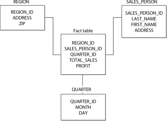
Figure 22-1 Example of the dimensional model: star schema

Each dimension table usually has a single-part primary key and several other attributes that describe this dimension closely. On the other hand, the primary key of the fact table is the combination of the primary keys of all dimension tables (see Figure 22-1). For this reason, the primary key of the fact table is made up of several foreign keys. (The number of dimensions also specifies the number of foreign keys in the fact table.) As you can see in Figure 22-1, the tables in a dimensional model build a star-like structure. Therefore, this model is often called star schema.

Another difference in the nature of data in a fact table and the corresponding dimension tables is that most nonkey columns in a fact table are numeric and additive, because such data can be used to execute necessary calculations. (Remember that a typical query on a data warehouse fetches thousands or even millions of rows at a time, and the only useful operation upon such a huge amount of rows is to apply an aggregate function, such as sum, maximum, or average.) For example, columns like Units_of_product_sold, Total_sales, Dollars_cost, or Profit are typical columns in the fact table. Such columns of the fact table are called measures.

On the other hand, columns of dimension tables are strings that contain textual descriptions of the dimension. For instance, columns such as Address, Location, and Name often appear in dimension tables. (These columns are usually used as headers in reports.) Another consequence of the textual nature of columns of dimension tables and their use in queries is that each dimension table contains many more indices than the corresponding fact table. (A fact table usually has only one unique index composed of all columns belonging to the primary key of that table.) Table 22-1 summarizes the differences between the fact table and dimension tables.

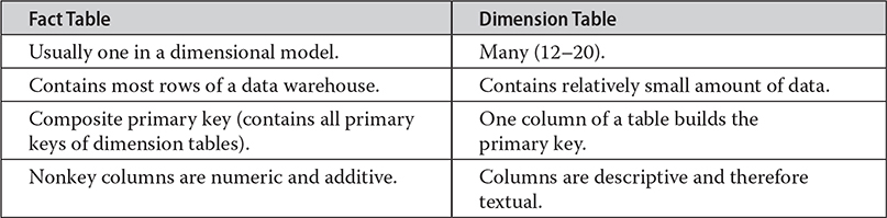
Table 22-1 Differences Between Fact Table and Dimension Tables

NOTE Sometimes it is necessary to have multiple fact tables in a data warehouse. If you have different sets of measures, each set has to be tied to a different fact table.

Columns of dimension tables are usually highly denormalized, which means that a lot of columns depend on each other. The denormalized structure of dimension tables has one important purpose: all columns of such a table are used as column headers in reports. If the denormalization of data in a dimension table is not desirable, a dimension table can be decomposed into several subtables. This is usually necessary when columns of a dimension table build hierarchies. (For example, the product dimension could have columns such as Product_id, Category_id, and Subcategory_id that build three hierarchies, with the primary key, Product_id, as the root.) This structure, in which each level of a base entity is represented by its own table, is called a snowflake schema. Figure 22-2 shows the snowflake schema of the product dimension.

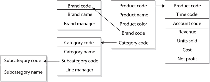
Figure 22-2 The snowflake schema of the product dimension

The extension of a star schema into a corresponding snowflake schema has some benefits (reduction of used disk space, for example) and one main disadvantage: the snowflake schema requires more join operations to get information from lookup tables, which negatively impacts performance. For this reason, the performance of queries based on the snowflake schema is generally slow. Therefore, the design using the snowflake schema is recommended only in a few very specialized cases.

Cubes and Their Architectures

BI systems support different types of data storage. Some of these data storage types are based on a multidimensional database that is also called a cube. A cube is a subset of data from the data warehouse that can be organized into multidimensional structures. To define a cube, you first select a fact table from the dimensional schema and identify numerical columns (measures) of interest within it. Then you select dimension tables that provide descriptions for the set of data to be analyzed. To demonstrate this, consider how the cube for car sales analysis might be defined. For example, the fact table may include the measures Cars_sold, Total_sales, and Costs, while the tables Models, Quarters, and Regions specify dimension tables. The cube in Figure 22-3 shows all three dimensions: Models, Regions, and Quarters.

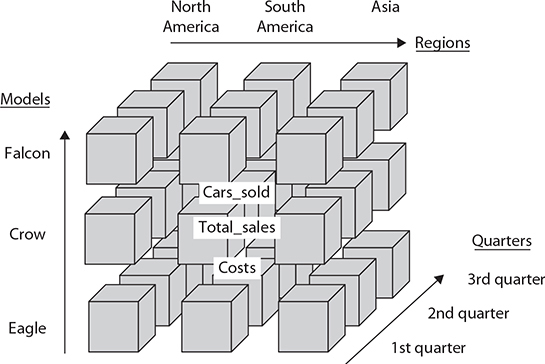
Figure 22-3 Cube with dimensions: Models, Quarters, and Regions

In each dimension there are discrete values called members. For instance, the Regions dimension may contain the following members: ALL, North America, South America, and Europe. (The ALL member specifies the total of all members in a dimension.)

Additionally, each cube dimension can have a hierarchy of levels that allows users to ask questions at a more detailed level. For example, the Regions dimension can include the following level hierarchies: Country, Province, and City. Similarly, the Quarters dimension can include Month, Week, and Day as level hierarchies.

NOTE Cubes and multidimensional databases are managed by special systems called multidimensional database systems (MDBMSs). SQL Server’s MDBMS is called Analysis Services, which is covered in Chapter 23.

The physical storage of a cube is described after the following discussion of aggregation.

Aggregation

Data is stored in the fact table in its most detailed form so that corresponding reports can make use of it. On the other hand (as stated earlier), a typical query on a fact table fetches thousands or even millions of rows at a time, and the only useful operation upon such a huge amount of rows is to apply an aggregate function (sum, maximum, or average). This different use of data can reduce performance of ad hoc queries if they are executed on low-level (atomic) data, because time- and resource-intensive calculations will be necessary to perform each aggregate function. For this reason, low-level data from the fact table should be summarized in advance and stored in intermediate tables. Because of their “aggregated” information, such tables are called aggregate tables, and the whole process is called aggregation.

NOTE An aggregate row from the fact table is always associated with one or more aggregate dimension table rows. For example, the dimensional model in Figure 22-1 could contain the following aggregate rows: monthly sales aggregates by salespersons by region and region-level aggregates by salespersons by day.

An example will show why low-level data should be aggregated. An end user may want to start an ad hoc query that displays the total sales of the organization for the last month. This would cause the server to sum all sales for each day in the last month. If an average of 500 sales transactions occur per day in each of 500 stores of the organization, and data is stored at the transaction level, this query would have to read 7,500,000 (500 × 500 × 30 days) rows and build the sum to return the result. Now consider what happens if the data is aggregated in a table that is created using monthly sales by store. In this case, the table will have only 500 rows (the monthly total for each of 500 stores), and the performance gain will be dramatic.

How Much to Aggregate?

Concerning aggregation, there are two extreme solutions: no aggregation at all, and exhaustive aggregation for every possible combination of queries that users will need. From the preceding discussion, it should be clear that no aggregation at all is out of the question, because of performance issues. (The data warehouse without any aggregation table probably cannot be used at all as a production data store.) The opposite solution is also not acceptable, for several reasons:

•   Enormous amount of disk space needed to store additional data

•   Overwhelming maintenance of aggregate tables

•   Initial data load too long

Storing additional data that is aggregated at every possible level consumes an additional amount of disk space that increases the initial disk space by a factor of six or more (depending on the amount of the initial disk space and the number of queries that users will need). The creation of tables to hold the aggregates for all existing combinations is an overwhelming task for the system administrator. Finally, building aggregates at initial data load can have devastating results if this load already lasts for a long time and the additional time is not available.

From this discussion you can see that aggregate tables should be carefully planned and created. During the planning phase, keep these two main considerations in mind when determining what aggregates to create:

•   Where is the data concentrated?

•   Which aggregates would most improve performance?

The planning and creation of aggregate tables is dependent on the concentration of data in the columns of the base fact table. In a data warehouse, where there is no activity on a given day, the corresponding row is not stored at all. So if the system loads a large number of rows, as compared to the number of all rows that can be loaded, aggregating by that column of the base fact table improves performance enormously. In contrast, if the system loads few rows, as compared to the number of all rows that can be loaded, aggregating by that column is not efficient.

Here is another example to demonstrate the preceding discussion. For products in the grocery store, only a few of them (say, 15 percent) are actually sold on a given day. If we have a dimensional model with three dimensions, Product, Store, and Time, only 15 percent of the combination of the three corresponding primary keys for the particular day and for the particular store will be occupied. The daily product sales data will thus be sparse. In contrast, if all or many products in the grocery store are sold on a given day (because of a special promotion, for example), the daily product sales data will be dense.

To find out which dimensions are sparse and which are dense, you have to build rows from all possible combinations of tables and evaluate them. Usually, the Time dimension is dense, because there are always entries for each day. Given the dimensions Product, Store, and Time, the combination of the Store and Time dimensions is dense, because for each day there will certainly be data concerning selling in each store. On the other hand, the combination of the Store and Product dimensions is sparse (for the reasons previously discussed). In this case, the dimension Product is generally sparse, because its appearance in combination with other dimensions is sparse.

The choice of aggregates that would most improve performance depends on end users. Therefore, at the beginning of a BI project, you should interview end users to collect information on how data will be queried, how many rows will be retrieved by these queries, and other criteria.

Physical Storage of a Cube

Online analytical processing (OLAP) systems usually use one of the following three different architectures to store multidimensional data:

•   Relational OLAP (ROLAP)

•   Multidimensional OLAP (MOLAP)

•   Hybrid OLAP (HOLAP)

Generally, these three architectures differ in the way in which they store leaf-level data and precomputed aggregates. (Leaf-level data is the finest grain of data that is defined in the cube’s measure group. Therefore, the leaf-level data corresponds to the data of the cube’s fact table.)

In ROLAP, the precomputed data isn’t stored. Instead, queries access data from the relational database and its tables in order to bring back the data required to answer the question. MOLAP is a type of storage in which the leaf-level data and its aggregations are stored using a multidimensional cube.

Although the logical content of these two storage types is identical for the same data warehouse, and both ROLAP and MOLAP analytic tools are designed to allow analysis of data through the use of the dimensional data model, there are some significant differences between them. The advantages of the ROLAP storage type are as follows:

•   Data is not duplicated.

•   Materialized (that is, indexed) views can be used for aggregation.

If the data should also be stored in a multidimensional database, a certain amount of data must be duplicated. Therefore, the ROLAP storage type does not need additional storage to copy the leaf-level data. Also, the calculation of aggregation can be executed very quickly with ROLAP if the corresponding summary tables are generated using indexed views.

On the other hand, MOLAP also has several advantages over ROLAP:

•   Aggregates are stored in a multidimensional form.

•   Query response is generally faster.

Using MOLAP, many aggregates are precomputed and stored in a multidimensional cube. That way the system does not have to calculate the result of such an aggregate each time it is needed. In the case of MOLAP, the database engine and the database itself are usually optimized to work together, so the query response may be faster than in ROLAP.

HOLAP storage is a combination of the MOLAP and ROLAP storage types. Precomputed data is stored as in the case of the MOLAP storage, while the leaf-level data is left in the relational database. (Therefore, for queries using aggregation, HOLAP is identical to MOLAP.) The advantage of HOLAP storage is that the leaf-level data is not duplicated.

Data Access

Data in a data warehouse can be accessed using three general techniques:

•   Reporting

•   OLAP

•   Data mining

Reporting is the simplest form of data access. A report is just a presentation of a query result in a tabular form. (Reporting is discussed in detail in Chapter 25.) With OLAP, you analyze data interactively; that is, it allows you to perform comparisons and calculations along any dimension in a data warehouse.

NOTE Transact-SQL supports all standardized functions and constructs in relation to SQL/OLAP. This topic will be discussed in detail in Chapter 24.

Data mining is used to explore and analyze large quantities of data in order to discover significant patterns. This discovery is not the only task of data mining: using this technique, you must be able to turn the existing data into information and turn the information into action. In other words, it is not enough to analyze data; you have to apply the results of data mining meaningfully and take action upon the given results. (Data mining, as the most complex of the three techniques, will not be covered in this introductory book.)

Summary

At the beginning of a BI project, the main question is what to build: a data warehouse or a data mart. Probably the best answer is to start with one or more data marts that can later be united in a data warehouse. Most of the existing tools in the BI market support this alternative.

In contrast to operational databases that use ER models for their design, the design of data warehouses is best done using a dimensional model. These two models show significant differences. If you are already acquainted with the ER model, the best way to learn and use the dimensional model is to forget everything about the ER model and start modeling from scratch.

After this introductory discussion of general considerations about the BI process, the next chapter discusses the server part of Microsoft Analysis Services.

Exercises

E.22.1   Discuss the differences between OLTP and analytic systems.

E.22.2   Discuss the differences between the ER and dimensional models.

E.22.3   A data warehouse project starts with the ETL (extracting, transforming, loading) process. Explain the three subprocesses.

E.22.4   Discuss the differences between a fact table and corresponding dimension tables.

E.22.5   Discuss the benefits of the three storage types: MOLAP, ROLAP, and HOLAP.

E.22.6   Why is it necessary to aggregate data stored in a fact table?