CHAPTER |
|
26 |
Optimizing Techniques for Data Warehousing |
In This Chapter
This chapter describes three optimizing techniques pertaining to data warehousing. The first part of this chapter discusses when it is reasonable to store all entity instances in a single table and when it is better, for performance reasons, to partition the table’s data. After a general introduction to data partitioning and the type of partitioning supported by the Database Engine, the steps that you have to follow to partition your table(s) are discussed in detail. You will then be given some partitioning techniques that can help increase system performance, followed by a list of important suggestions for how to partition your data and indices.
The second part of this chapter explains the technique called star join optimization. Two examples are presented to show you in which cases the query optimizer uses this technique instead of the usual join processing techniques. The role of bitmap filters will be explained, too.
The last part of this chapter describes an alternative form of a view, called an indexed view (or materialized view). This form of view materializes the corresponding query and allows you to achieve significant performance gains in relation to queries with aggregated data.
NOTE All the techniques described in this chapter can be applied only to relational OLAP (ROLAP).
Data Partitioning
The easiest and most natural way to design an entity is to use a single table. Also, if all instances of an entity belong to a table, you don’t need to decide where to store its rows physically, because the database system does this for you. For this reason there is no need for you to do any administrative tasks concerning storage of table data, if you don’t want to.
On the other hand, one of the most frequent causes of poor performance in relational database systems is contention for data that resides on a single I/O device. This is especially true if you have one or more very large tables with millions of rows. In that case, on a system with multiple CPUs, partitioning the table can lead to better performance through parallel operations.
By using data partitioning, you can divide very large tables (and indices too) into smaller parts that are easier to manage. This allows many operations to be performed in parallel, such as loading data and query processing.
Partitioning also improves the availability of the entire table. By placing each partition on its own disk, you can still access one part of the entire data even if one or more disks are unavailable. In that case, all data in the available partitions can be used for read and write operations. The same is true for maintenance operations.
If a table is partitioned, the query optimizer can recognize when the search condition in a query references only rows in certain partitions and therefore can limit its search to those partitions. That way, you can achieve significant performance gains, because the query optimizer has to analyze only a fraction of data from the partitioned table.
NOTE In this chapter, I discuss only horizontal table partitioning. Vertical partitioning is also an issue, but it does not have the same significance as horizontal partitioning.
How the Database Engine Partitions Data
A table can be partitioned using any column of the table. Such a column is called the partition key. (It is also possible to use a group of columns for the particular partition key.) The values of the partition key are used to partition table rows to different filegroups.
Two other important notions in relation to partitioning are the partition scheme and partition function. The partition scheme maps the table rows to one or more filegroups. The partition function defines how this mapping is done. In other words, the partition function defines the algorithm that is used to direct the rows to their physical location.
The Database Engine supports only one form of partitioning, called range partitioning. Range partitioning divides table rows into different partitions based on the value of the partition key. Hence, by applying range partitioning you will always know in which partition a particular row will be stored.
NOTE Besides range partitioning, there are several other forms of horizontal partitioning. One of them is called hash partitioning. In contrast to range partitioning, hash partitioning places rows one after another in partitions by applying a hashing function to the partition key. Hash partitioning is not supported by the Database Engine.
The steps for creating partitioned tables using range partitioning are described next.
Steps for Creating Partitioned Tables
Before you start to partition database tables, you have to complete the following steps:
1. Set partition goals.
2. Determine the partition key and number of partitions.
3. Create a filegroup for each partition.
4. Create the partition function and partition scheme.
5. Create partitioned indices (optionally).
All of these steps will be explained in the following sections.
Set Partition Goals
Partition goals depend on the type of applications that access the table that should be partitioned. There are several different partition goals, each of which could be a single reason to partition a table:
• Improved performance for individual queries
• Reduced contention
• Improved data availability
If your primary goal of table partitioning is to improve performance for individual queries, then distribute all table rows evenly. That way, the database system doesn’t have to wait for data retrieval from a partition that has more rows than other partitions. Also, if such queries access data by performing a table scan against significant portions of a table, then you should partition the table rows only. (Partitioning the corresponding index will just add overhead in such a case.)
Data partitioning can reduce contention when many simultaneous queries perform an index scan to return just a few rows from a table. In this case, you should partition the table and index with a partition scheme that allows each query to eliminate unneeded partitions from its scan. To reach this goal, start by investigating which queries access which parts of the table. Then partition table rows so that different queries access different partitions.
Partitioning improves the availability of the database. By placing each partition on its own filegroup and locating each filegroup on its own disk, you can increase the data availability, because if one disk fails and is no longer accessible, only the data in that partition is unavailable. While the system administrator services the corrupted disk, limited access still exists to other partitions of the table.
Determine the Partition Key and Number of Partitions
A table can be partitioned using any table column. The values of the partition key are used to partition table rows to different filegroups. For the best performance, each partition should be stored in a separate filegroup, and each filegroup should be stored on a separate disk device. By spreading the data across several disk devices, you can balance the I/O and improve query performance, availability, and maintenance.
You should partition the data of a table using a column that does not frequently change. If you use a column that is often modified, any update operation of that column can force the system to move the modified rows from one partition to the other, and this could be time consuming.
Create a Filegroup for Each Partition
To achieve better performance, higher data availability, and easier maintenance, use different filegroups to separate table data. The number of filegroups to use depends mostly on the hardware you have. When you have multiple CPUs, partition your data so that each CPU can access data on one disk device. If the Database Engine can process multiple partitions in parallel, the processing time of your application will be significantly reduced.
Each data partition must map to a filegroup. To create a filegroup, you use either the CREATE DATABASE statement or ALTER DATABASE statement. Example 26.1 shows the creation of a database called test_partitioned with one primary filegroup and two other filegroups.
NOTE Before you create the test_partitioned database, you have to change the physical addresses of all .mdf and .ndf files in Example 26.1 according to the file system you have on your computer.
Example 26.1
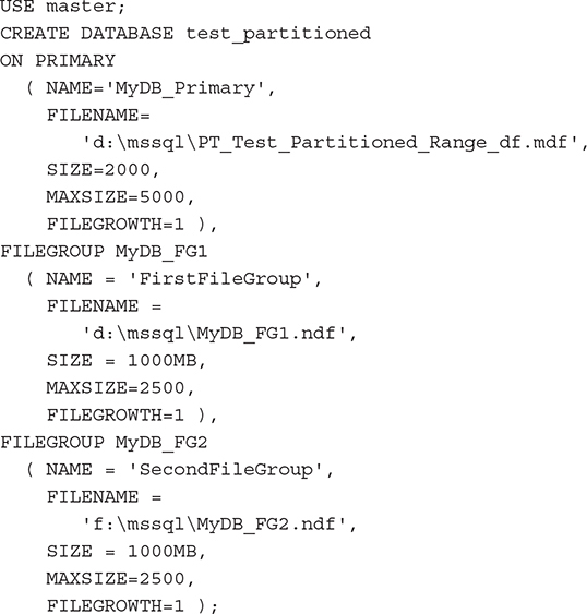
Example 26.1 creates a database called test_partitioned, which contains a primary filegroup, MyDB_Primary, and two other filegroups, MyDB_FG1 and MyDB_FG2. The MyDB_FG1 filegroup is stored on the D: drive, while the MyDB_FG2 filegroup is stored on the F: drive.
If you want to add filegroups to an existing database, use the ALTER DATABASE statement. Example 26.2 shows how to create another filegroup for the test_partitioned database.
Example 26.2
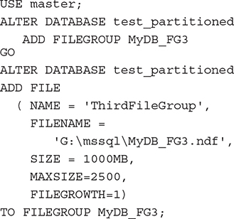
Example 26.2 uses the ALTER DATABASE statement to create an additional filegroup called MyDB_FG3 on the G: drive. The second ALTER DATABASE statement adds a new file to the created filegroup. Notice that the TO FILEGROUP option specifies the name of the filegroup to which the new file will be added.
Create the Partition Function and Partition Scheme
The next step after creating filegroups is to create the partition function, using the CREATE PARTITION FUNCTION statement. The syntax of the CREATE PARTITION FUNCTION is as follows:
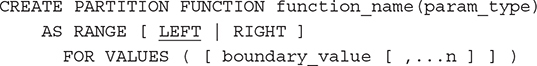
function_name defines the name of the partition function, while param_type specifies the data type of the partition key. boundary_value specifies one or more boundary values for each partition of a partitioned table or index that uses the partition function.
The CREATE PARTITION FUNCTION statement supports two forms of the RANGE option: RANGE LEFT and RANGE RIGHT. RANGE LEFT determines that the boundary condition is the upper boundary in the first partition. According to this, RANGE RIGHT specifies that the boundary condition is the lower boundary in the last partition (see Example 26.3). If not specified, RANGE LEFT is the default.
Example 26.3 shows the definition of the partition function.
Example 26.3
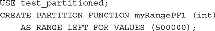
The myRangePF1 partition function specifies that there will be two partitions and that the boundary value is 500,000. This means that all values of the partition key that are less than or equal to 500,000 will be placed in the first partition, while all values greater than 500,000 will be stored in the second partition. (Note that the boundary value is related to the values in the partition key.)
The created partition function is useless if you don’t associate it with specific filegroups. As mentioned earlier in the chapter, you make this association via a partition scheme, and you use the CREATE PARTITION SCHEME statement to specify the association between a partition function and the corresponding filegroups. Example 26.4 shows the creation of the partition scheme for the partition function in Example 26.3.
Example 26.4
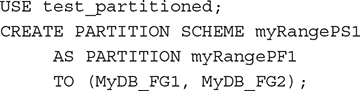
Example 26.4 creates the partition scheme called myRangePS1. According to this scheme, all values to the left of the boundary value (i.e., all values < 500,000) will be stored in the MyDB_FG1 filegroup. Also, all values to the right of the boundary value will be stored in the MyDB_FG2 filegroup.
NOTE When you define a partition scheme, you must be sure to specify a filegroup for each partition, even if multiple partitions will be stored on the same filegroup.
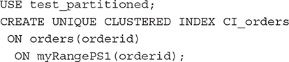
The creation of a partitioned table is slightly different from the creation of a nonpartitioned table. As you might guess, the CREATE TABLE statement must contain the name of the partition scheme and the name of the table column that will be used as the partition key. Example 26.5 shows the enhanced form of the CREATE TABLE statement that is used to define partitioning of the orders table.
Example 26.5
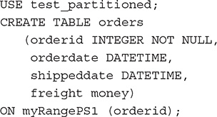
The ON clause at the end of the CREATE TABLE statement is used to specify the already-defined partition scheme (see Example 26.4). The specified partition scheme ties together the column of the table (orderid) with the partition function where the data type (INT) of the partition key is specified (see Example 26.3).
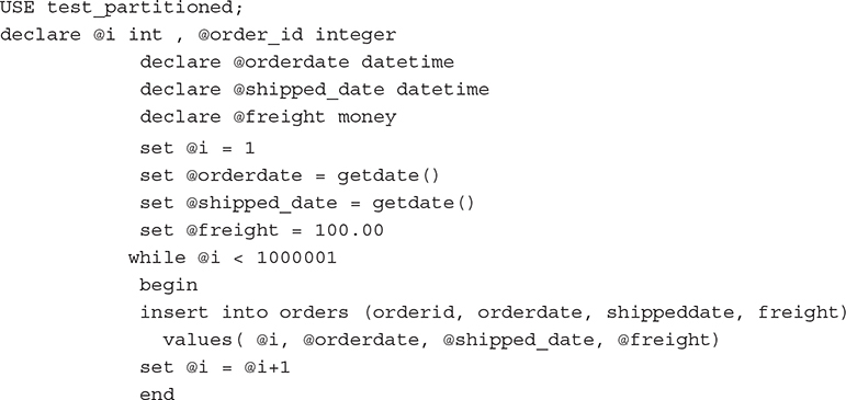
The batch in Example 26.6 loads a million rows into the orders table. You can use the sys.partitions view to edit the information concerning partitions in the orders table.
Example 26.6
Create Partitioned Indices
When you partition table data, you can partition the indices that are associated with that table, too. You can partition table indices using the existing partition scheme for that table or a different one. When both the indices and the table use the same partition function and the same partitioning columns (in the same order), the table and index are said to be aligned. When a table and its indices are aligned, the database system can move partitions in and out of partitioned tables very effectively, because the partitioning of both database objects is done with the same algorithm. For this reason, in the most practical cases it is recommended that you use aligned indices.
Example 26.7 shows the creation of a clustered index for the orders table. This index is aligned because it is partitioned using the partition scheme of the orders table.
Example 26.7
As you can see from Example 26.7, the creation of the partitioned index for the orders table is done using the enhanced form of the CREATE INDEX statement. This form of the CREATE INDEX statement contains an additional ON clause that specifies the partition scheme. If you want to align the index with the table, specify the same partition scheme as for the corresponding table. (The first ON clause is part of the standard syntax of the CREATE INDEX statement and specifies the column for indexing.)
Partitioning Techniques for Increasing System Performance
The following partitioning techniques can significantly increase performance of your system:
• Table collocation
• Partition-aware seek operation
• Parallel execution of queries
Table Collocation
Besides partitioning a table together with the corresponding indices, the Database Engine also supports the partitioning of two tables using the same partition function. This partition form means that rows of both tables that have the same value for the partition key are stored together at a specific location on the disk. This concept of data partitioning is called collocation.
Suppose that, besides the orders table (see Example 26.3), there is also an order_details table, which contains zero, one, or more rows for each unique order ID in the orders table. If you partition both tables using the same partition function on the join columns orders.orderid and order_details.orderid, the rows of both tables with the same value for the orderid columns will be physically stored together. Suppose that there is a unique order with the identification number 49031 in the orders table and five corresponding rows in the order_details table. In the case of collocation, all six rows will be stored side by side on the disk. (The same procedure will be applied to all rows of these tables with the same value for the orderid columns.)
This technique has significant performance benefits when, accessing more than one table, the data to be joined is located at the same partition. In that case the system doesn’t have to move data between different data partitions.
Partition-Aware Seek Operation
The internal representation of a partitioned table appears to the query processor as a composite (multicolumn) index with an internal column as the leading column. (This column, called partitionedID, is a hidden computed column used internally by the system to represent the ID of the partition containing a specific row.)
For example, suppose there is a tab table with three columns, col1, col2, and col3. (col1 is used to partition the table, while col2 has a clustered index.) The Database Engine treats internally such a table as a nonpartitioned table with the schema tab (partitionID, col1, col2, col3) and with a clustered index on the composite key (partitionedID, col2). This allows the query optimizer to perform seek operations based on the computed column partitionID on any partitioned table or index. That way, the performance of a significant number of queries on partitioned tables can be improved because the partition elimination is done earlier.
Parallel Execution of Queries
The Database Engine supports execution of parallel threads. In relation to this feature, the system provides two query execution strategies on partitioned objects:
• Single-thread-per-partition strategy The query optimizer assigns one thread per partition to execute a parallel query plan that accesses multiple partitions. One partition is not shared between multiple threads, but multiple partitions can be processed in parallel.
• Multiple-threads-per-partition strategy The query optimizer assigns multiple threads per partition regardless of the number of partitions to be accessed. In other words, all available threads start at the first partition to be accessed and scan forward. As each thread reaches the end of the partition, it moves to the next partition and begins scanning forward. The thread does not wait for the other threads to finish before moving to the next partition.
Which strategy the query optimizer chooses depends on your environment. It chooses the single-thread-per-partition strategy if queries are I/O-bound and include more partitions than the degree of parallelism. It chooses the multiple-threads-per-partition strategy in the following cases:
• Partitions are striped evenly across many disks.
• Your queries use fewer partitions than the number of available threads.
• Partition sizes differ significantly within a single table.
Editing Information Concerning Partitioning
You can use the following catalog views to display information concerning partitioning:
• sys.partitions
• sys.partition_schemes
• sys.partition_functions
The sys.partitions view contains a row for each partition of all the tables and some types of indices in the particular database. (All tables and indices in the Database Engine contain at least one partition, whether or not they are explicitly partitioned.)
The following are the most important columns of the sys.partitions catalog view:
• partition_id Specifies the partition ID, which is unique within the current database.
• object_id Defines the ID of the object to which this partition belongs.
• index_id Indicates the ID of the index within that object.
• hobt_id Indicates the ID of the data heap or B-tree that contains the rows for this partition.
• partition_number Indicates a 1-based partition number within the owning index or heap. For nonpartitioned tables and indices, the value of the partition_number column is 1.
Example 26.8 displays a list of all partitioned tables in the test_partitioned database.
Example 26.8
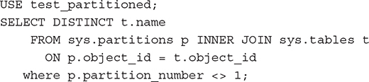
The result is

In Example 26.8 the sys.partitions catalog view is joined with sys.tables to get the list of all partitioned tables. Note that if you are looking specifically for partitioned tables, then you will have to filter your query with the condition
![]()
because for nonpartitioned tables, the value of the partition_number column is always 1.
The sys.partition_schemes catalog view contains a row for each data space with type = PS (“partition scheme”). (Generally, the data space can be a filegroup, partition scheme, or FILESTREAM data filegroup.) This view inherits the columns from the sys.data_spaces catalog view.
The sys.partition_functions catalog view contains a row for each partition function belonging to an instance of the Database Engine. The most important columns are name and function_id. The name column specifies the name of the partition function. (This name must be unique within the database.) The function_id column defines the ID of the corresponding partition function. This value is unique within the database.
Example 26.9 shows the use of the sys.partition_functions catalog view.
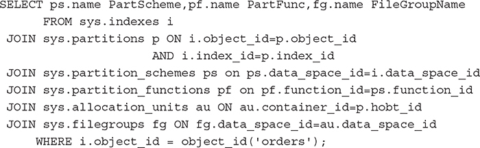
Example 26.9
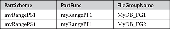
For the orders table of the test_partitioned database, find the name of the corresponding partition scheme as well as the name of the partition function used by that scheme. Additionally, display names of all filegroups associated with that partition function.
The result is
Example 26.9 joins six catalog views to obtain the desired information: sys.indexes, sys.partitions, sys.partition_schemes, sys.partition_functions, sys.allocation_units, and sys.filegroups. To join sys.indexes with sys.partitions, we use the combination of the values of the object_id and index_id columns. Also, the join operation between sys.indexes and sys.partition_schemes is done using the data_space_id column in both tables. (data_space_id is an ID value that uniquely specifies the corresponding data space.)
sys.partition_functions and sys.partition_schemes are connected using the function_id column in both tables. sys.filegroups and sys.allocation_units are joined together using the already mentioned column data_space_id. Finally, to join the sys.partitions and sys.allocation_units views, we use the hobt_id column from the former and the container_id column from the latter. (For the description of the hobt_id column, see the definition of the sys.partitions view earlier in this section.)
Guidelines for Partitioning Tables and Indices
The following suggestions are guidelines for partitioning tables and indices:
• Do not partition every table. Partition only those tables that are accessed most frequently.
• Consider partitioning a table if it is a huge one, meaning it contains at least several hundred thousand rows.
• For best performance, use partitioned indices to reduce contention between sessions.
• Balance the number of partitions with the number of processors on your system. If it is not possible for you to establish a 1:1 relationship between the number of partitions and the number of processors, specify the number of partitions as a multiple factor of the number of processors. (For instance, if your computer has four processors, the number of partitions should be divisible by four.)
• Do not partition the data of a table using a column that changes frequently. If you use a column that changes often, any update operation of that column can force the system to move the modified rows from one partition to another, and this could be very time consuming.
• For optimal performance, partition the tables to increase parallelism, but do not partition their indices. Place the indices in a separate filegroup.
Star Join Optimization
As you already know from Chapter 22, the star schema is a general form for structuring data in a data warehouse. A star schema usually has one fact table, which is connected to several dimension tables. The fact table can have 100 million rows or more, while dimension tables are fairly small relative to the size of the corresponding fact table. Generally, in decision support queries, several dimension tables are joined with the corresponding fact table. The convenient way for the query optimizer to execute such queries is to join each of the dimension tables used in the query with the fact table, using the primary/foreign key relationship. Although this technique is the best one for numerous queries, significant performance gains can be achieved if the query optimizer uses special techniques for particular groups of queries. One such specific technique is called star join optimization.
Before you start to explore this technique, take a look at how the query optimizer executes a query in the traditional way, as shown in Example 26.10.
Example 26.10
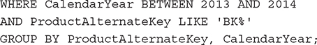
The execution plan of Example 26.10 is shown in Figure 26-1.
As you can see from the execution plan in Figure 26-1, the query joins first the FactInternetSales fact table with the DimDate dimension table using the relationship between the primary key in the dimension table (DateKey) and the foreign key in the fact table (DateKey). After that, the second dimension table, DimProduct, is joined with the result of the previous join operation. Both join operations use the hash join method.
Figure 26-1 Execution plan of Example 26.10
The use of the star join optimization technique will be explained using Example 26.11.
Example 26.11
The query optimizer uses the star join optimization technique only when the fact table is very large in relation to the corresponding dimension tables. To ensure that the query optimizer would apply the star join optimization technique, I significantly enhanced the FactInternetSales fact table from the AdventureWorksDW database. The original size of this table is approximately 64,000 rows, but for this example I created an additional 500,000 rows by generating random values for the ProductKey, SalesOrderNumber, and SalesOrderLineNo columns. Figure 26-2 shows the execution plan of Example 26.11.
The query optimizer detects that the star join optimization technique can be applied and evaluates the use of bitmap filters. (A bitmap filter is a small to midsize set of values that is used to filter data. Bitmap filters are always stored in memory.)
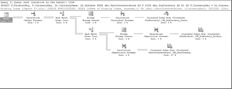
Figure 26-2 Execution plan of Example 26.11
As you can see from the execution plan in Figure 26-2, the fact table is first scanned using the corresponding clustered index. After that the bitmap filters for both dimension tables are applied. (Their task is to filter out the rows from the fact table.) This has been done using the hash join technique. At the end, the significantly reduced sets of rows from both streams are joined together.
NOTE Do not confuse bitmap filters with bitmap indices! Bitmap indices are persistent structures used in BI as an alternative to B+-tree structures. The Database Engine doesn’t support bitmap indices.
Indexed Views
As you already know from Chapter 10, there are several special index types. One of them is the indexed view, the topic of this section.
A view always contains a query that acts as a filter. Without indices created for a particular view, the Database Engine builds dynamically the result set from each query that references a view. (“Dynamically” means that if you modify the content of a table, the corresponding view will always show the new information.) Also, if the view contains computations based on one or more columns of the table, the computations are performed each time you access the view.
Building dynamically the result set of a query can decrease performance if the view with its SELECT statement processes many rows from one or more tables. If such a view is frequently used in queries, you could significantly increase performance by creating a clustered index on the view (demonstrated in the next section). Creating a clustered index means that the system materializes the dynamic data into the leaf pages on an index structure.
The Database Engine allows you to create indices on views. Such views are called indexed (or materialized) views. When a unique clustered index is created on a view, the view is executed and the result set is stored in the database in the same way a base table with a clustered index is stored. This means that the leaf nodes of the clustered index’s B+-tree contain data pages (see also the description of the clustered table in Chapter 10).
NOTE Indexed views are implemented through syntax extensions to the CREATE INDEX and CREATE VIEW statements. In the CREATE INDEX statement, you specify the name of a view instead of a table name. The syntax of the CREATE VIEW statement is extended with the SCHEMABINDING clause. For more information on extensions to this statement, see the description in Chapter 11.
Creating an Indexed View
Creating an indexed view is a two-step process:
1. Create the view using the CREATE VIEW statement with the SCHEMABINDING clause.
2. Create the corresponding unique clustered index.
Example 26.12 shows the first step, the creation of a typical view that can be indexed to gain performance. (This example assumes that works_on is a very large table.)
Example 26.12
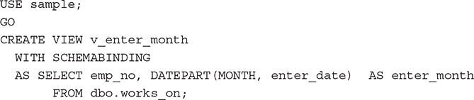
The works_on table in the sample database contains the enter_date column, which represents the starting date of an employee in the corresponding project. If you want to retrieve all employees that entered their projects in a specified month, you can use the view in Example 26.12. To retrieve such a result set using index access, the Database Engine cannot use a table index, because an index on the enter_date column would locate the values of that column by the date, and not by the month. In such a case, indexed views can help, as Example 26.13 shows.
Example 26.13
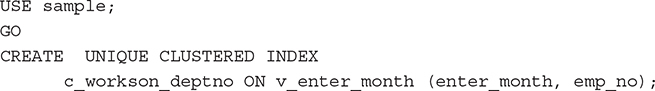
To make a view indexed, you have to create a unique clustered index on the column(s) of the view. (As previously stated, a clustered index is the only index type that contains the data values in its leaf pages.) After you create that index, the database system allocates storage for the view, and then you can create any number of nonclustered indices because the view is treated as a (base) table.
An indexed view can be created only if it is deterministic—that is, the view always displays the same result set. In that case, the following options of the SET statement must be set to ON:
• QUOTED_IDENTIFIER
• CONCAT_NULL_YIELDS_NULL
• ANSI_NULLS
• ANSI_PADDING
• ANSI_WARNINGS
Also, the NUMERIC_ROUNDABORT option must be set to OFF.
There are several ways to check whether the options in the preceding list are appropriately set, as discussed in the upcoming section “Editing Information Concerning Indexed Views.”
To create an indexed view, the view definition has to meet the following requirements:
• All referenced (system and user-defined) functions used by the view have to be deterministic—that is, they must always return the same result for the same arguments.
• The view must reference only base tables.
• The view and the referenced base table(s) must have the same owner and belong to the same database.
• The view must be created with the SCHEMABINDING option. SCHEMABINDING binds the view to the schema of the underlying base tables.
• The referenced user-defined functions must be created with the SCHEMABINDING option.
• The SELECT statement in the view cannot contain the following clauses and options: DISTINCT, UNION, TOP, ORDER BY, MIN, MAX, COUNT, SUM (on a nullable expression), subqueries, derived tables, or OUTER.
The Transact-SQL language allows you to verify all of these requirements by using the IsIndexable parameter of the objectproperty property function, as shown in Example 26.14. If the value of the function is 1, all requirements are met and you can create the clustered index.
Example 26.14
![]()
Modifying the Structure of an Indexed View
To drop the unique clustered index on an indexed view, you have to drop all nonclustered indices on the view, too. After you drop its clustered index, the view is treated by the system as a traditional one.
NOTE If you drop an indexed view, all indices on that view are dropped.
If you want to change a standard view to an indexed one, you have to create a unique clustered index on it. To do so, you must first specify the SCHEMABINDING option for that view. You can drop the view and re-create it, specifying the SCHEMABINDING clause in the CREATE SCHEMA statement, or you can create another view that has the same text as the existing view but a different name.
NOTE If you create a new view with a different name, you must ensure that the new view meets all the requirements for an indexed view that are described in the preceding section.
Editing Information Concerning Indexed Views
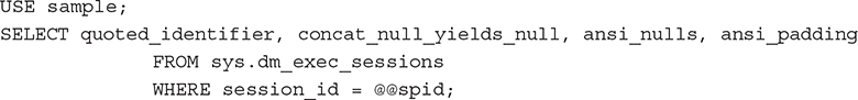
You can use the sessionproperty property function to test whether one of the options of the SET statement is activated (see the earlier section “Creating an Indexed View” for a list of the options). If the function returns 1, the setting is ON. Example 26.15 shows the use of the function to check how the QUOTED_IDENTIFIER option is set.
Example 26.15
![]()
The easier way is to use the dynamic management view called sys.dm_exec_sessions, because you can retrieve values of all options discussed previously using only one query. (Again, if the value of a column is 1, the corresponding option is set to ON.) Example 26.16 returns the values for the first four SET statement options from the list in “Creating an Indexed View.” (The global variable @@spid is described in Chapter 4.)
Example 26.16
The sp_spaceused system procedure allows you to check whether the view is materialized—that is, whether or not it uses the storage space. The result of Example 26.17 shows that the v_enter_month view uses storage space for the data as well as for the defined index.
Example 26.17
![]()
The result is

Benefits of Indexed Views
Besides possible performance gains for complex views that are frequently referenced in queries, the use of indexed views has two other advantages:
• The index of an indexed view can be used even if the view is not explicitly referenced in the FROM clause.
• All modifications to data are reflected in the corresponding indexed view.
Probably the most important property of indexed views is that a query does not have to explicitly reference a view to use the index on that view. In other words, if the query contains references to columns in the base table(s) that also exist in the indexed views, and the optimizer estimates that using the indexed view is the best choice, it chooses the view indices in the same way it chooses table indices when they are not directly referenced in a query.
When you create an indexed view, the result set of the view (at the time the index is created) is stored on the disk. Therefore, all data that is modified in the base table(s) will also be modified in the corresponding result set of the indexed view.
Besides all the benefits that you can gain by using indexed views, there is also a (possible) disadvantage: indices on indexed views are usually more complex to maintain than indices on base tables, because the structure of a unique clustered index on an indexed view is more complex than the structure of the corresponding index on a base table.
The following types of queries can achieve significant performance benefits if a view that is referenced by the corresponding query is indexed:
• Queries that process many rows and contain join operations or aggregate functions
• Join operations and aggregate functions that are frequently performed by one or several queries
If a query references a standard view and the database system has to process many rows using the join operation, the optimizer will usually use a suboptimal join method. However, if you define a clustered index on that view, the performance of the query could be significantly enhanced, because the optimizer can use an appropriate method. (The same is true for aggregate functions.)
If a query that references a standard view does not process many rows, the use of an indexed view could still be beneficial if the query is used very frequently. (The same is true for groups of queries that join the same tables or use the same type of aggregates.)
Summary
The Database Engine supports range partitioning of data and indices that is entirely transparent to the application. Range partitioning partitions rows based on the value of the partition key. In other words, the data is divided using the values of the partition key.
If you want to partition your data, you must complete the following steps:
1. Set partition goals.
2. Determine the partition key and number of partitions.
3. Create a filegroup for each partition.
4. Create the partition function and partition scheme.
5. Create partitioned indices (if necessary).
By using different filegroups to separate table data, you achieve better performance, higher data availability, and easier maintenance.
The partition function is used to map the rows of a table or index into partitions based on the values of a specified column. To create a partition function, use the CREATE PARTITION FUNCTION statement. To associate a partition function with specific filegroups, use a partition scheme. When you partition table data, you can partition the indices associated with that table, too. You can partition table indices using the existing partition schema for that table or a different one.
Star join optimization is an index-based optimization technique that supports the optimal use of indices on huge fact tables. The main advantages of this technique are the following:
• Significant performance improvements in case of moderately and highly selective star join queries.
• No additional storage cost. The system does not create any new indices, but uses bitmap filters instead.
Indexed views are used to increase performance of certain queries. When a unique clustered index is created on a view, the view becomes materialized—that is, its result set is physically stored in the same way a content of a base table is stored.
The next chapter describes columnstore indices, another technique for storing content of tables.