WE’RE ONLY HUMAN

There is nothing so disastrous as a rational
investment policy in an irrational world.

—JOHN MAYNARD KEYNES

Sears is a legendary American success story. Sears began as a mail-order catalog selling everything from watches and toys to cars and ready-to-assemble houses and evolved into the nation’s largest retailer. Sears was in the Dow Jones Average for seventy-five years, but struggled in the 1990s to compete with discount retailers like Walmart, Target, and Home Depot. Sales and profits fell, and Sears stock price dropped nearly 50 percent between June and November 1999. Home Depot, on the other hand, was opening a new store every fifty-six hours. Its tools competed directly with the legendary Craftsman tools from Sears, and it was winning the battle. Home Depot’s stock rose 50 percent between June and November 1999. On November 1, 1999, Home Depot replaced Sears in the Dow Jones Industrial Average.

Sears stock subsequently outperformed Home Depot. It wasn’t a fluke and it wasn’t that Home Depot had been jinxed by being included in the Dow. It had everything to do with how stock prices are affected by human emotions that can leave $100 bills on the sidewalk. Let’s look at several examples.

ANCHORING

Anchoring is a general human tendency to rely on a reference point when making decisions. A student did a term paper in one of my statistics classes in which randomly selected students were asked one of these two questions:

The population of Bolivia is 5 million.

Estimate the population of Bulgaria.

The population of Bolivia is 15 million.

Estimate the population of Bulgaria.

Those who were told that Bolivia’s population was 15 million tended to give higher answers than did those told that Bolivia’s population was 5 million. Several similar questions confirmed this pattern. People use the known “fact” as an anchor for their guess.

When we buy a car, we tend to judge whether we are getting a good deal by comparing the final negotiated price to the dealer’s initial price, no matter how unrealistic the initial price. Thus, a good salesman starts the haggling with a high price.

In real estate, many people use the price they paid for their home as an anchor for its current value: “Our house can’t be worth $300,000; we bought it for $400,000.” This anchoring causes some homeowners to behave in ways that are, well, irrational.

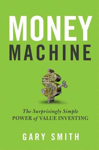
Figure 9-1 shows that the average price of condominiums in Boston nearly tripled between 1982 and 1988 and then fell by almost 35 percent over the next five years.

People who paid low prices for their condos in the early 1980s could make profits selling in the early 1990s, but people who bought in the late 1980s would have losses. A study found that sellers facing losses tended to ask higher prices for their condos. Not surprisingly, their high-priced condos went unsold. These condo owners were using their purchase price as an anchor for what their condos were worth and were so averse to taking a loss that they would rather not sell.

This behavior was not rational. There is no reason why condos purchased during a time of high prices are worth more than condos purchased during a time of low prices. It certainly makes no difference to buyers. If it makes a difference to sellers, they pay for their irrationality by not being able to sell their condos.

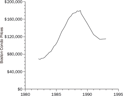
People also use anchoring to gauge whether interest rates are high or low. A family I know (I’ll call them Greg and Jane Landon) bought their first house in Eugene, Oregon, in 1971. Figure 9-2 shows that going back to at least 1920, mortgage rates had never been above 6 percent until they broke the 6 percent barrier in 1966 and hit 7.5 percent in 1971.

Greg thought they should wait to buy a home until mortgage rates went back to “normal” levels; that is, below 6 percent. Greg was using past mortgage rates as an anchor to gauge what mortgage rates should be.

But interest rates aren’t governed by physical laws, like gravity or magnetism, that force them to behave in easily predictable ways. Just because mortgage rates had been 6 percent in the past doesn’t mean they will be 6 percent in the future. Jane persuaded Greg that they should buy a home to call their own. Greg grimaced and they borrowed at 7.5 percent to buy a starter home. (In real estate, that’s a euphemism for small.)

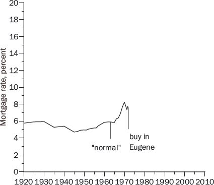
Seven years later, in 1978, they moved to Houston, Texas, and mortgage rates were now 9.6 percent (see Figure 9-3).

Greg was even more certain that they should wait for mortgage rates to return to normal. But the value of their Oregon home had doubled and, at that time, sellers had to pay a 35 percent capital gains tax on the profit they made from their homes, unless they purchased a new home—in which case the capital gain was rolled over and the tax was deferred, perhaps indefinitely. So Greg gritted his teeth and they bought a home in Houston with a 9.6 percent mortgage.

Three years later, in 1981, they moved to Seattle. Now they would have to pay capital gains taxes on their Eugene and Houston homes unless they bought another house. Unfortunately, mortgage rates were now above 17 percent (Figure 9-4).

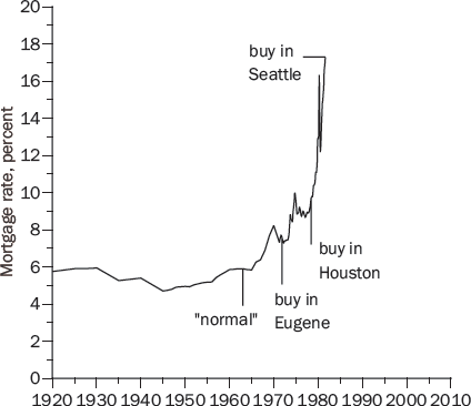
Fortunately, Greg’s new company had an employee mortgage plan that would lend them money at 8.7 percent. Greg was much happier with 8.7 percent than with 17 percent, but he thought they would be even better off if they waited for mortgage rates to return to normal. The deciding factor was the annoying capital gains tax they would have to pay if they didn’t buy. So, they bought a home in Seattle with an 8.7 percent mortgage.

Finally, in 2003 mortgage rates fell below 6 percent (Figure 9-5). Mortgage rates had returned to normal, just as Greg had predicted! But it took forty years. If the Landons had waited to buy a home until mortgage rates went back to 6 percent, they would have missed out on the best investments they made in their entire lives: their homes in Eugene, Houston, and Seattle.

One moral of this story is, don’t try to time the real estate market. Another is to watch out for anchors that might sink you.

SUNK COSTS

You buy a colossal ice cream sundae for a special price but, halfway through, you’re feeling sick. Do you finish the sundae because you want to eat what you paid for? The relevant question is not how much you paid, but whether you would be better off eating the rest of the ice cream or throwing it away.

You have season tickets to college football games in the Midwest. Come November, the team sucks and the weather is worse. Do you go to games because you already paid for the tickets? The relevant question is whether you would be happier at the game or somewhere else.

There is nothing to be gained and much to be lost by moping about things you can’t change. Things that can’t be changed are called sunk costs. The ice cream sundae you bought but would get sick finishing is a sunk cost. So are tickets to a miserable football game. So is the price you paid for a stock. Yet many investors are reluctant to sell losers, despite the tax benefit, because selling for a loss is an admission that they made a mistake buying the stock in the first place.

In the early 1980s a famous Yale professor boasted to a friend of mine that he made 25 percent a year during the terrible bear market in the 1970s. Surely, my friend asked, you must have bought some stocks that went down? He nearly fell out of his chair laughing when the Yale professor replied, “Yes, but I haven’t sold them yet!” Then my friend realized that the professor was not trying to be funny.

The price you pay for a stock is a sunk cost. We should think about whether a stock is cheap or expensive at its current price, not whether the price is higher or lower than the price we paid, but it is hard to forget that sunk cost.

A BREAKEVEN MENTALITY

Daniel Kahneman and Amos Tversky observed that betting on long shots at horse races picks up toward the end of the day, presumably because people are looking for a cheap opportunity to win back what they lost earlier in the day. They argued that a “person who has not made peace with his losses is likely to accept gambles that would be unacceptable to him otherwise.”

Two students and I looked at the strategies used by experienced Texas Hold ’Em poker players. We found that most played looser after a big loss (betting so that they could stay in with hands they would normally fold). They evidently remembered their big losses and were eager to win back what they had lost.

Is this riskier play punished? It seems likely that experienced players generally use sound strategies, and that any changes are a mistake. That’s what happened. Players who played looser after a big loss were less successful than they were with their normal playing style.

If investors are like poker players, they may be tempted to make long-shot investments to recoup losses. A February 2009 article in the Wall Street Journal reported that many investors were responding to their stock market losses by making increasingly risky investments:

The financial equivalent of a “Hail Mary pass”—the desperate attempt, far from the goal line and late in a losing game, to fling the football as hard and as high as you can, hoping it will somehow come down for a score and wipe out your deficit.

Try not to let a breakeven mentality lure you into Hail Mary investments.

REGRESSION TO THE MEAN

Horace Secrist had a distinguished career as a professor of economics at Northwestern University. He wrote thirteen textbooks and was director of Northwestern’s Bureau of Economic Research. In 1933, in the depths of the national economic tragedy that became known as the Great Depression, he published a book that he hoped would explain the cause, provide solutions, and secure his legacy.

Secrist and his assistants spent ten years collecting and analyzing data for seventy-three different industries, including department stores, clothing stores, hardware stores, railroads, and banks. He compiled annual data for the years 1920 to 1930 on several metrics of business success, including the ratios of profits to sales and profits to assets. For each ratio, he divided the companies in an industry into quartiles based on the 1920 values of the ratio: the top 25 percent, the second 25, the third 25, and the bottom 25. He then calculated the average ratio from 1920 to 1930 for the stocks in each 1920 quartile. He found that the companies in the top two quartiles in 1920 were more nearly average in 1930, and that the companies in the bottom two quartiles in 1920 were also more nearly average in 1930.

He had evidently discovered a universal economic truth. American business was converging to mediocrity. His book documenting his discovery was titled The Triumph of Mediocrity in Business. The book was a statistical tour de force, 468 pages long, with 140 tables and 103 charts, supporting his remarkable discovery.

Then a brilliant statistician named Harold Hotelling wrote a devastating review that politely but firmly demonstrated that Secrist had wasted ten years proving nothing at all. What Secrist became famous for was being fooled by regression toward the mean.

THE STATISTICAL FALLACY

I once did some research with a student on regression to the mean in baseball. Not 468 pages, but at least we recognized regression when we saw it. A referee for the journal that published our paper wrote:

There are few statistical facts more interesting than regression to the mean for two reasons. First, people encounter it almost every day of their lives. Second, almost nobody understands it.

The coupling of these two reasons makes regression to the mean one of the most fundamental sources of error in human judgment, producing fallacious reasoning in medicine, education, government, and, yes, even sports.

Yes, we encounter regression to the mean almost every day and, yes, almost nobody understands it. This is a lethal combination—as Secrist discovered.

To understand regression, suppose that 100 people are asked twenty questions about world history. Each person’s “ability” is what his or her average score would be on a large number of these tests. Some people have an ability of 90, some 80, and some near zero.

Someone with an ability of 80 will average 80, but is not going to get 80 percent correct on every test. Imagine a test bank with zillions of questions. By the luck of the draw, a person with an ability of 80 will know the answers to more than 80 percent of the questions on one test and to fewer than 80 percent on another test. A person’s score on any single test is an imperfect measure of ability.

What, if anything, can we infer from someone’s test score? A key insight is that a person whose test score is high relative to the others who took the test probably also had a high score relative to his or her own ability. Someone who scores in the 90th percentile could be someone of more modest ability (perhaps the 85th, 80th, or 75th percentile in ability) who did unusually well, or someone of higher ability (perhaps the 95th percentile in ability) who did poorly. The former is more likely because there are more people with ability below the 90th percentile than above it.

If this person’s ability is, in fact, below the 90th percentile, then when this person takes another test, his or her score will probably also be below the 90th percentile. Similarly, a person who scores well below average is likely to have had an off day and should anticipate scoring somewhat higher on another test. This tendency of people who score far from the mean to score closer to the mean on a second test is an example of regression toward the mean.

Regression does not imply that everyone will soon get the same score on history tests, only that scores fluctuate around ability.

SECRIST’S FOLLY

In the same way, Secrist’s study of successful and unsuccessful companies involved regression toward the mean. In any given year, the most successful companies are likely to have had more good luck than bad and to have done well not only relative to other firms, but also relative to their own long-run profitability. The opposite is true of the least successful companies. This is why the subsequent performance of the top and bottom companies is usually closer to the average company. At the same time, their places at the extremes are taken by other companies experiencing fortune or misfortune. These fluctuations do not mean that all companies will soon be mediocre. As Hotelling put it, Secrist “really prove[d] nothing more than that the ratios in question have a tendency to wander about.”

REGRESSION IN THE STOCK MARKET

In Against the Gods, a bestselling, prize-winning book, Peter Bernstein wrote:

The track records of professional investment managers are also subject to regression to the mean. There is a strong probability that the hot manager of today will be the cold manager of tomorrow, or at least the day after tomorrow, and vice versa. . . . [T]he wisest strategy is to dismiss the manager with the best track record and to transfer one’s assets to the manager who has been doing the worst; this strategy is no different from selling stocks that have risen the furthest and buying stocks that have fallen furthest.

Bernstein is wise, but this is not wisdom. The idea that the best will be worst and the worst will be best is the gambler’s fallacy that good luck makes bad luck more likely. It is false and it is not regression to the mean. Regression occurs because the managers with the best track records probably benefited from good luck and are consequently not as far above average in ability as they seem. If there is any skill to stock picking, the person with the best track record can be expected to outperform the person with the worst record, but not by as much next year as last year. If stock picking is all luck, you may as well pick managers randomly—or save money by not using a manager at all—but there is no reason to choose the worst manager.

SHRUNKEN EARNINGS PREDICTIONS ARE BETTER PREDICTIONS

There is regression to the mean in stocks, as well as managers. A natural tendency in the stock market, where investors hope to invest in the next IBM, Walmart, or Google, is to see a year or two of rapidly increasing earnings and assume many years of similar rapid growth. Regression teaches us that a company with earnings up by 20 percent this year (or over the past few years) is more likely to have experienced good luck than bad luck and, most likely, will regress toward the mean in the future, disappointing overly optimistic investors.

Something very similar is true of predicted earnings. The most optimistic predictions are more likely to be overly optimistic than to be excessively pessimistic, so the companies with the most optimistic forecasts probably won’t do as well as predicted.

Two colleagues and I investigated this reasoning. Regression relates to relative values. Our guiding principle was that firms whose growth rates are predicted to be far from the mean will probably have growth rates closer to the mean. So, we adjusted the analysts’ forecasts by shrinking them toward the average forecast for all companies. Our adjusted forecasts were more accurate than the analysts’ forecasts 70 percent of the time, which is better than a 2-to-1 margin.

We didn’t use spreadsheets to predict market share, revenue, expenses, and the like. We didn’t even look at the company names. We just downloaded the forecast earnings growth rates and shrunk them toward the overall mean, using a marvelous statistical formula known as Kelley’s equation, and we out-predicted the professional predictors.

If investors are paying attention to these professional analysts (or making similar predictions themselves), stock prices are likely to be too high for companies with optimistic forecasts and too low for those with pessimistic forecasts—mistakes that will be corrected when earnings regress to the mean. If this conjecture is correct, stocks with relatively pessimistic earnings predictions may outperform stocks with relatively optimistic predictions.

Five portfolios were formed each year based on the analysts’ predicted earning growth for the current fiscal year. The most optimistic portfolio consisted of the 20 percent of the stocks with the highest predicted growth. The most pessimistic portfolio contained the 20 percent with the lowest predicted growth. The stock returns were then calculated for each portfolio over the next twelve months. A similar procedure was used for the year-ahead earnings forecasts, but the stock returns were calculated over the next twenty-four months.

Table 9-1 shows the results. The pessimistic portfolios trounced the optimistic portfolios. It is hard to imagine that this trouncing reflects some kind of risk premium. The pessimistic portfolios were actually safer.

The most plausible explanation is that the market’s insufficient appreciation of regression to the mean is leaving $100 bills on the sidewalk.

DOW DELETIONS

The Dow Jones Industrial Average is an average of the prices of thirty blue-chip stocks that represent the most prominent companies in the United States. An Averages Committee periodically changes the stocks in the Dow, sometimes because a firm merges with another company or is taken over by another company. More often, though, a company has some tough years and is no longer considered to be a blue-chip stock. Such fallen companies are replaced by more successful companies; for example, a thriving Home Depot replaced a struggling Sears in 1999.

When a faltering company is replaced by a flourishing company, which stock do you think does better subsequently—the stock going into the Dow or the stock going out? If you take regression into account, the stock booted out of the Dow probably will do better than the stock that replaces it.

This is counterintuitive because it is tempting to confuse a great company with a great stock. LeanMean may have a long history of strong, stable profits. But is it a good investment? The answer depends on the stock’s price. Is it an attractive investment at $10 a share? $100? $1,000? There are prices at which the stock is too expensive. There are prices at which the stock is cheap. No matter how good the company, value investors need to know the stock’s price before deciding whether it is an attractive investment.

Regarding Dow additions and deletions, the question for value investors is not whether the companies going into the Dow are doing better than the companies they are replacing, but which stocks are better investments. The stocks going into and out of the Dow are all familiar companies that are closely watched by thousands of investors. In 1999, investors were well aware of the fact that Home Depot was doing great and Sears was doing poorly. Their stock prices surely reflected this knowledge. That’s why Home Depot’s stock was up 50 percent, while Sears was down 50 percent.

However, the regression argument suggests that the companies taken out of the Dow are generally not in as dire straits as their recent performance suggests and that the companies replacing them are generally not as stellar as they appear. If so, stock prices will often be unreasonably low for the stocks going out and undeservedly high for the stocks going in. When a company that was doing poorly regresses to the mean, its stock price will rise. When a company that was doing spectacularly regresses to the mean, its price will fall. This argument suggests that stocks deleted from the Dow will generally outperform stocks added to the Dow.

Sears was bought by Kmart in 2005, five-and-a-half years after it was kicked out of the Dow. If you bought Sears stock just after it was deleted from the Dow, your total return until its acquisition by Kmart would have been 103 percent. Over the same five-and-a-half-year period, an investment in Home Depot, the stock that replaced Sears, would have lost 22 percent. The S&P 500 index of stock prices during this period had a return of –14 percent. Sears had an above-average return after it left the Dow, while Home Depot had a below-average return after it entered the Dow. (The Kmart-Sears combination has been ugly, but that’s another story.)

Is this comparison of Sears and Home Depot an isolated incident or part of a systematic pattern of Dow deletions outperforming Dow additions? There were actually four substitutions in 1999. Home Depot, Microsoft, Intel, and SBC replaced Sears, Goodyear Tire, Union Carbide, and Chevron. Home Depot, Microsoft, Intel, and SBC are all great companies, but all four stocks did poorly over the next decade.

Suppose that on the day the four substitutions were made, November 1, 1999, you had invested $25,000 in each of the four stocks added to the Dow, for a total investment of $100,000. This is your Addition Portfolio. You also formed a Deletion Portfolio by investing $25,000 in each of the stocks deleted from the Dow.

After ten years, the S&P 500 was down 23 percent. The Addition Portfolio did even worse, down 34 percent. The Deletion Portfolio, in contrast, was up 64 percent.

Maybe 1999 was an unusual year and substitutions made in other years turned out differently? Nope. In 2006 I did a study with two of my students of all fifty changes in the Dow back to October 1, 1928, when the Dow 30-stock average began; we found that deleted stocks did better than the stocks that replaced them in thirty-two cases and did worse in eighteen cases. A portfolio of deleted stocks beat a portfolio of added stocks by about 4 percent a year, which is a huge difference compounded over seventy-eight years. A $100,000 portfolio of added stocks would have grown to $160 million by 2006; a $100,000 portfolio of deleted stocks would have grown to $3.3 billion. The companies doing so poorly that they were booted out of the Dow have been better investments than the darlings that replaced them.

Our findings contradict the efficient market hypothesis since changes in the composition of the Dow are widely reported and well known. Once again, it seems that the market’s neglect of regression is leaving $100 bills on the sidewalk.

WOULD A STOCK BY ANY OTHER TICKER SMELL AS SWEET?

Several companies have shunned the traditional name-abbreviation convention and chosen ticker symbols that are memorable for their cheeky cleverness. Southwest Airlines’ choice of LUV as its ticker symbol was related to its efforts to brand itself as an airline “built on love.” Southwest is based at Dallas Love Field and has an open-seating policy that reportedly can lead to romance between strangers who sit next to each other. Its onboard snacks were originally called “love bites” and its drinks “love potions,” and a Southwest spokesman boasted about the number of romances that started on Southwest flights: “At times, we feel that we are the love brokers of the sky.”

Perhaps a clever ticker symbol is an indicator that a firm’s managers are smart and creative, with a sense of humor. On the other hand, wary investors may interpret a clever symbol as a silly marketing ploy by a company that feels it must resort to gimmicks to attract investor attention. Perhaps a clever symbol is a signal of desperation rather than intelligence.

Another possibility is that clever ticker symbols matter because they are memorable. There is considerable evidence that human judgments are shaped by how easily information is processed and remembered:

1.Objects shown for longer periods of time or with greater background contrast are rated more favorably.

2.Statements like “Osorno is in Chile” are more likely to be judged true if written in colors that are easier to read.

3.Aphorisms that rhyme are more likely to be judged true; for example, “Woes unite foes” versus “Woes unite enemies.”

These arguments suggest that ticker symbols that are easily processed and recalled might be rated favorably. For example, an investor might look at pet-related companies and come across VCA Antech, which operates a network of animal hospitals and diagnostic laboratories. A ticker symbol VCAA might pass unnoticed. But the actual ticker symbol, WOOF, is memorable. Perhaps a few days, weeks, or months later, this investor decides to invest in a pet-related company and remembers the symbol WOOF. (In a weird coincidence, it was a former student of mine who thought up the ticker WOOF.)

Two students and I looked at whether ticker symbols matter. Because cleverness is in the eye of the beholder, we used a survey to identify ticker symbols that people consider witty. First, we sifted through 33,000 ticker symbols for past and present companies, looking for ticker symbols that might be considered noteworthy. Ninety-three percent of our selections coincided. We merged the lists and discarded ticker symbols that were simply an abbreviation of the company’s name (BEAR for Bear Automotive Service Equipment and GLAD for Gladstone Capital) and kept symbols that showed ingenuity (GRRR for Lion Country Safari parks and MOO for United Stockyards).

We distributed 100 surveys with our culled list of 358 ticker symbols, the company names, and a brief description of each company’s business. We intentionally excluded seasoned investment professionals whose choices might have been influenced by the investment performance of the companies on the list.

For each trading day from the beginning of 1984 (when clever ticker symbols started becoming popular) to the end of 2005, we calculated the daily return for a portfolio of the clever-ticker stocks that received the most votes in our survey. Figure 9-6 shows that the clever-ticker portfolio lagged behind the market portfolio slightly until 1993 and then spurted ahead. Overall, the compounded annual returns were 24 percent for the clever-ticker portfolio and 12 percent for the market portfolio.

The market-beating performance was not because the clever-ticker stocks were concentrated in one industry. Our eighty-two clever-ticker companies span thirty-one of the eighty-one industry categories used by the U.S. government, with the highest concentration being eight companies in eating and drinking places, of which four beat the market and four did not. Nor was it due to the extraordinary performance of a small number of clever-ticker stocks: 65 percent of the clever-ticker stocks beat the market.

We do not know why these stocks did so well. Perhaps a clever ticker is a useful barometer of the managers’ ability, which reveals itself over time as the firm repeatedly exceeds investors’ expectations. Or perhaps a clever ticker matters because it is memorable and has a subtle but persistent influence on investors who buy the stock. Either way, it’s an unexpected $100 bill on the sidewalk.

IF HUMANS AREN’T AS SMART AS COMPUTERS

If humans are, well, human with human emotions, frailties, and inconsistencies, should we turn our investment decisions over to computers? Computers don’t have emotions, and well-written software doesn’t have inconsistencies. True enough, but computers don’t have common sense, either. Computers can identify statistical patterns but cannot gauge whether there is a logical basis for the discovered patterns.

When a statistical correlation between gold and silver prices was discovered in the 1980s, how could a computer possibly discern whether there was a sensible basis for this statistical correlation? In the 1990s, Long-Term Capital Management was bankrupted by a number of bets on correlations that did not have a persuasive explanation; for example, relationships among various French and German interest rates. A manager later lamented that “we had academics who came in with no trading experience and they started modeling away. Their trades might look good given the assumptions they made, but they often did not pass a simple smell test.”

Humans do make mistakes, leaving profitable opportunities for others, but humans also have the potential to recognize those mistakes and to avoid being seduced by patterns that lead computers astray.

Part II will give several detailed examples of how value investors can use the principles discussed in Part I to be successful investors.