
10
Testing and Profiling
CERTIFICATION OBJECTIVES
• Testing Applications with JUnit
Q&A Self Test
This chapter delves into two important topics that that are too often overlooked: unit testing and profiling. Unit tests are used to verify the basic functionality of an application. Profiling is an operation like debugging, except instead of looking at current stack values and tracing execution flow, the profiler monitors performance and provides tools for identifying and measuring CPU and memory use.
To facilitate unit testing, NetBeans supports JUnit and includes wizards for creating new unit tests and test suites. It also provides an integrated user interface for running and debugging the tests. Starting in NetBeans 6.0 NetBeans integrated a profiler into the IDE. The profiler was based on the JFluid research project from SunLabs. With this advanced profiler, profiling can be turned on and off dynamically while an application is running. Thus, large applications where profiling wasn’t feasible can now be analyzed. The type of profiling, either CPU or memory, can be changed without restarting the target application. The NetBeans Profiler supports profiling both local and remote Java applications. A NetBeans project is not required in order to profile an application. The profiler can capture data in snapshots for later analysis. For heap snapshots, NetBeans includes HeapWalker and supports searching the heap using the Object Query Language (OQL).
The NetBeans certification exam covers both JUnit testing and profiling desktop applications. Mastering these tools helps you build repeatable processes and takes the mystery out of application performance problems.
CERTIFICATION OBJECTIVE: Testing Applications with JUnit
Exam Objective 6.1 Demonstrate the ability to work with JUnit tests in the IDE, such as creating JUnit tests and interpreting JUnit test output.
Unit testing is the verification of individual code segments that an application comprises. A code segment can be a method, interface, class, or some piece of functionality. The granularity of the tests is up to the developer. The objective is to split an application into pieces and verify the correctness of the pieces. Once unit tests have been written, they can be periodically or regularly rerun to verify bug fixes and to validate core functionality as code evolves. Unit tests thus become the foundation of a regression test suite.
JUnit is the ubiquitous unit test framework for the Java platform and has been a testing mainstay for the past decade. Although JUnit test cases are written using standard Java classes, NetBeans includes custom user interfaces to expedite development and execution as well as to monitor the tests. NetBeans also isolates the source and classpath for unit tests so that test code doesn’t pollute the application. Leveraging the support within NetBeans, unit tests can be easily written and frequently run. NetBeans also supports the continuous integration server Hudson (http://hudson-ci.org). Hudson jobs can be kicked off within NetBeans and thus run the entire unit test suite.
The following topics are covered in this section:
![]() Understanding JUnit Basics and Versions
Understanding JUnit Basics and Versions
![]() Creating JUnit Tests and Suites
Creating JUnit Tests and Suites
![]() Managing Testing Classpath
Managing Testing Classpath
![]() Running JUnit Tests
Running JUnit Tests
![]() Configuring Continuous Integration Support
Configuring Continuous Integration Support
Understanding JUnit Basics and Versions
The premise of JUnit is fairly simple: write small nuggets of code to test basic units of functionality. The objective is to test the pieces of the application and verify that they work independently. While the application may not work as a whole, at least there is confidence and verification that the basic application building blocks work correctly. Ideally the unit test cases should be written prior to the actual implementation. Verifying that the building blocks work together is the province of integration testing
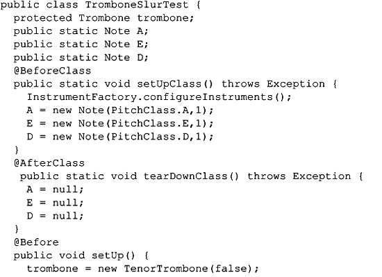
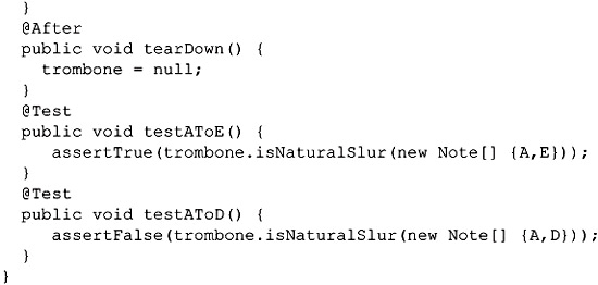
A unit test in JUnit is a regular Java class with several methods that perform the testing. Methods that prepare the test environment and post process can be optionally implemented. JUnit provides assert methods, different from the Java language asserts, to test conditions and terminate the test upon failure. Listing 10-1 shows a simple unit test from the MusicCoach application. This unit test has two test methods that are marked with the @Test annotation. It has two class-level setup and teardown methods and two instance-level setup and teardown methods: setUpClass, tearDownClass, setUp, and tearDown, respectively.
LISTING 10-1 TromboneSlurTest.java
Unit tests can then be grouped into test suites that can be run as entire units. Test suites can include other test suites to form a hierarchical structure. Listing 10-2 shows a simple test suite for trombones in the MusicCoach application. It ties the TromboneTest and TromboneSlurTest into one suite.
@RunWith(Suite.class)
@Suite.SuiteClasses({net.cuprak.music.instruments.
TromboneSlurTest.class,
net.cuprak.music.instruments.TromboneTest.class})
public class TromboneTestSuite {
@BeforeClass
public static void setUpClass() throws Exception {
// Do nothing
}
@AfterClass
public static void tearDownClass() throws Exception {
// Do nothing
}
}
Listings 10-1 and 10-2 target JUnit version 4. NetBeans supports two versions of JUnit: JUnit 3.x and 4.x. In NetBeans 6.8, JUnit 3.8.4 and 4.5 are preconfigured by default. JUnit 4 employs annotations to mark tests and eliminate the need for subclassing and naming conventions. Consequently JUnit 4 requires Java 5. Since there are many legacy applications, JUnit 3 is still supported. An application can make use of both JUnit 3 and JUnit 4 test classes, but a test class cannot mix versions, because tests and setup code will not execute as expected. JUnit 3 test cases must extend TestCase, and a test suite must extend TestSuite. JUnit 3 also lacks support for setUpClass and tearDownClass. In-depth discussion of the differences between JUnit 3 and 4 is outside the scope of this book. More information on the subject and links can be found at www.junit.org. JUnit 4 code samples in Listings 10-1 and 10-2 were back-ported to JUnit 3 in Listing 10-3.
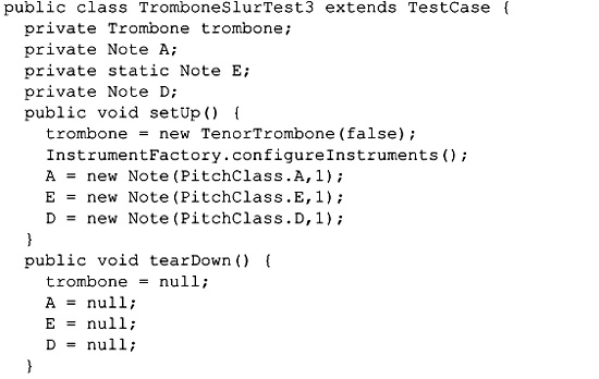
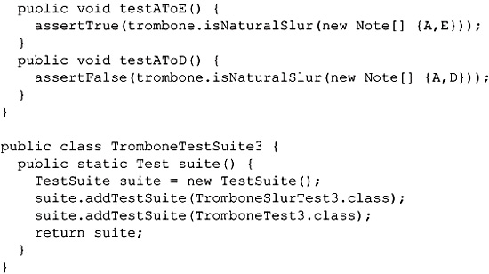
Table 10-1 lists the Java annotations available in JUnit 4.5. Many of these annotations were used in the code listings.
TABLE 10-1 Java 4.5 Annotations
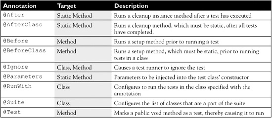
Know the difference between JUnit 3.x and 4.x. Also, NetBeans asks only once which version of JUnit should be used for a project. To update to a newer version, the new library must be added in Test Libraries of Project Properties. It also can be edited by right-clicking Test Libraries in the Projects window. This is a major feature of NetBeans’ JUnit support and will be touched upon in the exam.
Creating JUnit Tests and Suites
A new JUnit test or test suite is created by choosing File | New File (CTRL-N) and selecting a project template from the JUnit category. The available choices are shown in Figure 10-1. This dialog box can also be opened by right-clicking and choosing New | Other. The New File dialog box presents the following three options:
FIGURE 10-1 JUnit file templates
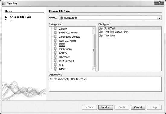
![]() JUnit Test Creates an empty JUnit test.
JUnit Test Creates an empty JUnit test.
![]() Test For Existing Class Creates a simple JUnit test case for testing methods of a single class.
Test For Existing Class Creates a simple JUnit test case for testing methods of a single class.
![]() Test Suite Creates a test suite for all tests in a selected Java test package.
Test Suite Creates a test suite for all tests in a selected Java test package.
Creating an Empty JUnit Test
Choosing the first option shown in Figure 10-1 and clicking Next displays the panel shown in Figure 10-2. This panel prompts for the basic information necessary to create an empty unit test:
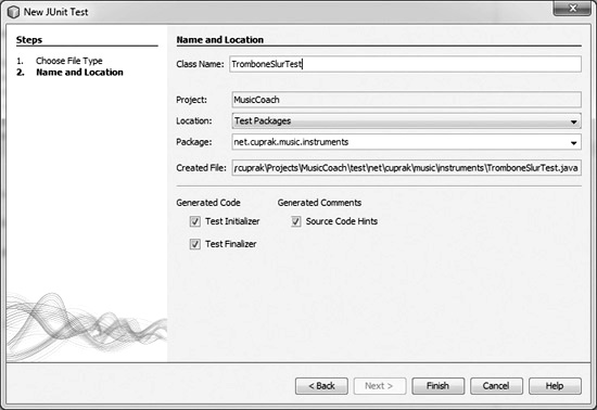
![]() Class Name The name of the test class to create.
Class Name The name of the test class to create.
![]() Project Non-editable field displaying the project to which the new JUnit class is added.
Project Non-editable field displaying the project to which the new JUnit class is added.
![]() Location Drop-down list of test source code packages that can be selected.
Location Drop-down list of test source code packages that can be selected.
![]() Package The package of the new JUnit class. It can be edited or selected.
Package The package of the new JUnit class. It can be edited or selected.
![]() Created File Non-editable field displaying the full path to the generated file.
Created File Non-editable field displaying the full path to the generated file.
![]() Generated Code Generates the following types of setup methods:
Generated Code Generates the following types of setup methods:
![]() Test Initializer Creates a skeleton public void setUp() method.
Test Initializer Creates a skeleton public void setUp() method.
![]() Test Finalizer Creates a skeleton public void tearDown() method.
Test Finalizer Creates a skeleton public void tearDown() method.
![]() Generated Comments Only option available is Source Code Hints, which are comments directing you to the code to implement.
Generated Comments Only option available is Source Code Hints, which are comments directing you to the code to implement.
Once these options are populated, NetBeans creates a new JUnit skeleton. A project can possess one or more test classpaths, hence the drop-down list for Location.
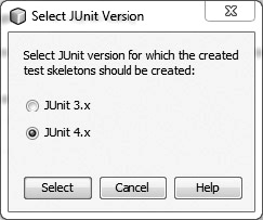
The first time a JUnit test class is created for a project, NetBeans prompts for the JUnit version to be used. The dialog box that appears is shown in Figure 10-3. NetBeans only asks this question the first time a JUnit test class is created. If JUnit 3 has been chosen, the project can be switched to JUnit 4 by adding the JUnit 4.x library to the project in Project Properties.
FIGURE 10-3 Select JUnit Version
Creating a JUnit for Existing Class
Choosing the Test For Existing Class option (in the New File dialog box under File Types) displays the panel in Figure 10-4. This New Test For Existing Class dialog box can also be displayed by selecting a class in the Projects window and pressing CTRL-SHIFT-U or right-clicking and choosing Tools | Create JUnit Tests. This panel is used to create JUnit test classes for existing classes and interfaces. NetBeans introspects the class and generates skeleton methods. It is your job to implement each one of these methods. By default, each skeleton test method fails until implemented. This ensures that you do not forget to write a test.
FIGURE 10-4 New Test For Existing Class
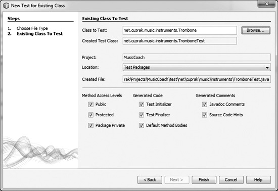
The configuration parameters in this panel include:
![]() Class To Test The class to be tested.
Class To Test The class to be tested.
![]() Created Test Class The name of the test class to create.
Created Test Class The name of the test class to create.
![]() Project Non-editable field displaying the project to which the new JUnit class is added.
Project Non-editable field displaying the project to which the new JUnit class is added.
![]() Location Drop-down list of test source code packages that can be selected.
Location Drop-down list of test source code packages that can be selected.
![]() Created File Non-editable field displaying the full path to the generated file.
Created File Non-editable field displaying the full path to the generated file.
![]() Method Access Levels Selecting a level causes NetBeans to generate skeleton code for all of the methods matching the access level. Access levels are Public, Protected, and Package Private.
Method Access Levels Selecting a level causes NetBeans to generate skeleton code for all of the methods matching the access level. Access levels are Public, Protected, and Package Private.
![]() Generated Code Generates the following types of setup methods:
Generated Code Generates the following types of setup methods:
![]() Test Initializer Creates a skeleton public void setUp() method.
Test Initializer Creates a skeleton public void setUp() method.
![]() Test Finalizer Creates a skeleton public void tearDown() method.
Test Finalizer Creates a skeleton public void tearDown() method.
![]() Default Method Bodies For skeleton test methods, inserts the following code: fail("The test case is a prototype.");
Default Method Bodies For skeleton test methods, inserts the following code: fail("The test case is a prototype.");
![]() Generated Comments Selecting either of the following options generates the respective comments:
Generated Comments Selecting either of the following options generates the respective comments:
![]() Javadoc Comments Adds Javadoc to the test method. Note that Javadoc is not automatically generated for the setup/teardown methods.
Javadoc Comments Adds Javadoc to the test method. Note that Javadoc is not automatically generated for the setup/teardown methods.
![]() Source Code Hints Adds a TODO comment in the skeleton test methods.
Source Code Hints Adds a TODO comment in the skeleton test methods.
For JUnit 4, NetBeans automatically generates the following two methods:
![]()
and
![]()
These two methods are respectively executed before any of the tests have been run and after all of the tests have been run. These two methods are created regardless of the settings in Figure 10-4.
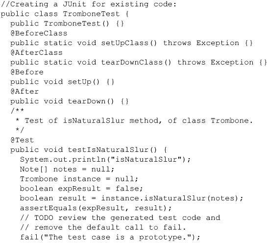
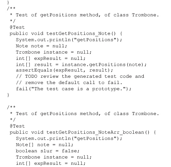
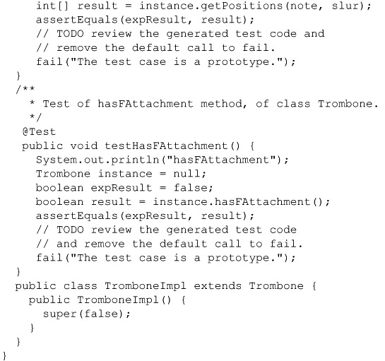
Listing 10-4 is a sample JUnit test for an existing class. Accepting the defaults in Figure 10-4 created this class. JUnit 4.x was selected as the JUnit version. Test methods are annotated with @Test. NetBeans has attempted to create a reasonable skeleton structure for each test method. Each test method corresponds to a method in the target class. Note the fail(...) invocations in each method that will automatically fail the test.
LISTING 10-4 JUnit Test for Existing Class
Creating a Test Suite
JUnit test suites are used to run a group of tests together. Test suites can include other test suites. Choosing Test Suite in Figure 10-1 displays the New Test Suite panel in Figure 10-5. This panel prompts for the basic information necessary to create the test suite. Listing 10-2 is an example test suite created by NetBeans. By default, NetBeans scans a package looking for unit test cases to be added to the suite. The panel prompts for the following settings before generating the code:
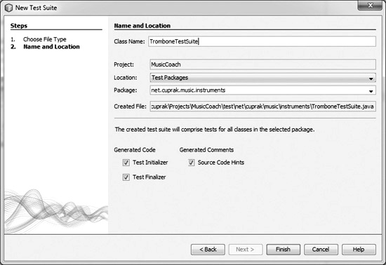
![]() Class Name Name of the test suite.
Class Name Name of the test suite.
![]() Project Non-editable field displaying the project to which the new JUnit class is added.
Project Non-editable field displaying the project to which the new JUnit class is added.
![]() Location Drop-down list of test source code packages that can be selected.
Location Drop-down list of test source code packages that can be selected.
![]() Package The package where the test suite is stored and also contains the JUnit test classes to be added to the suite.
Package The package where the test suite is stored and also contains the JUnit test classes to be added to the suite.
![]() Created File Non-editable field displaying the full path to the generated file.
Created File Non-editable field displaying the full path to the generated file.
![]() Generated Code Generates the following types of setup methods:
Generated Code Generates the following types of setup methods:
![]() Test Initializer Creates a skeleton public void setUp() method.
Test Initializer Creates a skeleton public void setUp() method.
![]() Test Finalizer Creates a skeleton public void tearDown() method.
Test Finalizer Creates a skeleton public void tearDown() method.
![]() Generated Comments Generates comments; in the case of a TestSuite, only the Source Code Hints option is available. Source code hints add a TODO comment in the skeleton methods.
Generated Comments Generates comments; in the case of a TestSuite, only the Source Code Hints option is available. Source code hints add a TODO comment in the skeleton methods.
NetBeans can also generate a test suite and unit tests for all the classes in a source package. Right-clicking a package under Source Packages in the Projects window and choosing Create JUnit Tests creates a test suite and JUnits for each class. This is a quick way to generate test skeletons for all of the classes in a package.
Managing Testing Classpaths
The test classpath for a project is configured in Project Properties for standard projects. A standard project is one that uses the NetBeans-provided build script. Project Properties can be accessed by either right-clicking the project in the Projects window or by choosing File | Project Properties. The dialog box is shown in Figure 10-6. Within Project Properties choose the Libraries category. The Compile Tests and Run Tests tabs configure the classpath for the unit tests. Projects, libraries, and other projects can be added as dependencies. These classpaths extend the compile classpath.
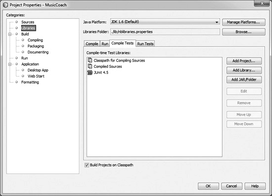
NetBeans maintains two separate classpaths so that references to JUnit or other classes used to support unit testing don’t creep into the main source code tree. This enforces a firewall between the application’s implementation and its test code. For example, it would be dangerous if mock objects, objects that simulate the behavior of objects in a controlled manner for testing, were inadvertently used in the production deployment.
Running JUnit Tests
JUnit tests and test suites are executed or debugged either in NetBeans or on the command line using the project’s Ant script. When testing is initiated, the Tests window opens; this window can be explicitly opened by choosing Window | Output | Test Results. Individual test methods can only be run from this window after all of the test methods have been executed.
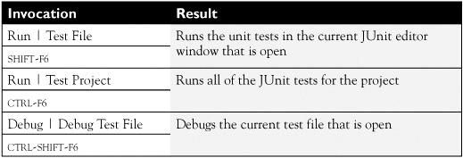
Table 10-2 lists the various methods for running either a single unit test or all of the tests in a project. In addition, right-clicking a JUnit test in the Projects window displays a context menu with Test File and Debug Test File.
TABLE 10-2 Unit Execution Options
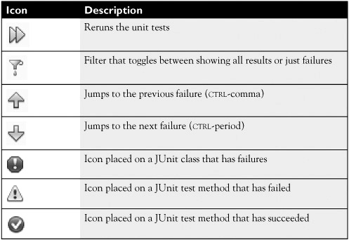
When a project is either executed or debugged in NetBeans, the Test Results window shown in Figure 10-7 opens. The window is divided into two panels, with the left side listing the JUnit tests executed and the right side displaying the standard out/error from the tests. A status bar indicates the percentage of tests that have either succeeded or failed. The number of tests that have succeeded and failed is listed below the status bar. A green “passed” represents a success, whereas a red “FAILED” represents a failure. Double-clicking a test method in the left panel jumps to the code for the test. An individual test can be rerun by right-clicking a test and selecting Run Again. Table 10-3 lists the icons along the left of the window as well as the glyphs on the unit tests denoting their status.
FIGURE 10-7 JUnit test execution
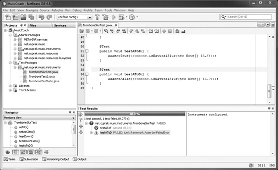
TABLE 10-3 Test Results Window Icons
JUnit tests can also be run from the command line. Whether running unit tests in the IDE or on the command line, the Ant script for the project is used. The unit tests can be executed in the project directory by entering ant test. This assumes that Ant is already installed. Ant executes the test method in build.xml, which is inherited from nbproject/build-impl.xml. Executing the test target causes the project to be built. If any unit tests fail, the build script fails execution.
NetBeans automatically outputs XML reports for the unit tests that it runs. These XML files are placed in the directory build/test/results. To reformat and generate a human-readable JUnit report, the test-report Ant target can be overridden in build.xml. The default implementation in nbproject/build-impl.xml contains an empty stub method for this purpose. The following example code, which should be added to build.xml, generates an HTML report:
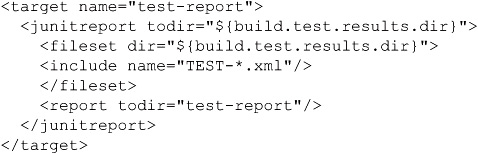

The Ant variables used in this snippet were defined in nbproject/project.properties. When you’re extending the Ant build, this is a good file to examine for existing Ant variables.
EXERCISE 10-1 Running Unit Tests
In this exercise, you are going to run the existing test suite for the Jmol application. In Chapter 3 you checked out Jmol and created a NetBeans project for it. Now you will run it and verify that all of its tests are running.
1. Open the Jmol project you created in Exercise 3-1.
2. Open Test Packages in the Projects window.
3. Open the org.jmol node to reveal the AllTests.java class.
4. Right-click AllTests.java and choose Test File. NetBeans now compiles the project and runs the test suite.
5. The Output window should open displaying the output of the build. If the Test Results window does not open automatically, choose Window | Output | Test Results.
6. Open the org.jmol.AllTests node to reveal all of the tests that were run along with their status. All tests should have passed.
7. Notice that the unit tests were written using JUnit 3.
EXERCISE 10-2 Creating a JUnit Test
In this exercise, you create a new JUnit test for an existing Jmol utility class.
1. Open the Jmol project you created in Exercise 3-1.
2. Choose File | New File and select Test For Existing Class from the templates available under the JUnit category. Click Next.
3. Select org.jmol.util.ArrayUtil for the Class To Test. You can enter this class directly, or click Browse and search for it.
4. Accept the other defaults and click Finish. The default generates a stub test method for each method in ArrayUtil.java.
5. NetBeans should now ask whether the project should use JUnit 3 or 4. Choose JUnit 3 because the other tests were written using JUnit 3, and we want to integrate this new test into the test suite.
6. Open the class org.jmol.AllTests.java, and add the following line to the end of the suite method:
![]()
7. Right-click AllTests.java in the Projects window and choose Test File. By default, the stub methods created by NetBeans will fail. This is intentional so that you don’t forget to implement the methods. Tests should fail until they are implemented.
8. Double-click a failure in the Test Results window to view that stub method.
9. Remove the assert and fail statements so that the test succeeds.
10. Right-click the failed test in the Test Results window, and choose Run Again to verify that the test now succeeds.
Configuring Continuous Integration Support
NetBeans supports Hudson, which is a continuous integration server. A continuous integration server like Hudson retrieves a project from source control on a regular basis and builds the project as well as runs the unit tests. Good JUnit tests are only useful if you run them regularly. NetBeans facilitates regular JUnit testing by tightly integrating Hudson into the IDE. Projects can be easily added to Hudson, and NetBeans will alert the developer when either the build or JUnits fail. For a large project it often isn’t feasible to run all of the JUnits on a developer’s desktop machine prior to committing the code. This tight integration with Hudson makes regularly running JUnit tests easy.
Hudson regularly retrieves a project from source control, builds it, and then runs the unit tests. Typically Hudson is configured to watch the version control and kick off a build when code is committed, usually with a time delay. Hudson can also be configured to do regular builds throughout the day or at night. Hudson not only builds the project but also executes the unit tests. Building and testing frequently ensures that bugs are caught early.
Hudson is an open source project and can be downloaded from http://hudson-ci.org. It is a Java web application and is deployed by dropping the WAR file into a Java web application container such as Tomcat or GlassFish. No other configuration is needed to start the application. After it is deployed, permissions can be configured so that not everyone can add, build, or view the results of a build/test. If the Hudson WAR file is dropped into the webapps directory of Apache Tomcat, Hudson can be monitored and managed locally at http://localhost:8080/hudson.
Continuous integration should involve not only building the code base and running the unit tests but also rebuilding the test environment. For example, database scripts should be run frequently, and the database schema regenerated to ensure that there is a repeatable process in place. Tools such as LiquiBase (www.liquibase.org) can be integrated into the build and test process.
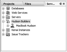
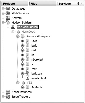
Hudson servers are managed in the Services window under Hudson Builders. An example is shown in Figure 10-8 with a remote Hudson server, MacBook Hudson, configured.
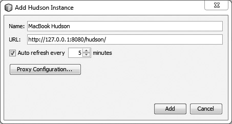
Servers that are already running can be mounted in NetBeans by right-clicking and choosing Add Hudson Instance. This displays the dialog box in Figure 10-9.
FIGURE 10-9 Add Hudson Instance
Right-clicking and selecting New Build adds new Hudson jobs. Only applications that are being managed by version control can be added. Once an application is added, the Hudson instance can be opened to display the list of applications, as shown in Figure 10-10. The artifacts from the build can be opened and inspected as well as the JUnit reports.
FIGURE 10-10 Application under Hudson
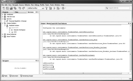
NetBeans checks Hudson at regular intervals for updates on jobs. NetBeans is watching for build failures due to either compilation errors or JUnits. A popup for the MusicCoach application is shown in Figure 10-11. Here we can see a warning that the unit tests have failed. Clicking the link for Some Tests Failed opens the Output window for the JUnit test execution. This is shown in Figure 10-12.
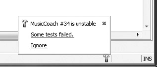
FIGURE 10-12 Hudson JUnit output
EXERCISE 10-3 Unit Testing with Hudson
In this exercise, you deploy and configure Hudson. You then create a Hudson job that regularly checks out and builds Jmol.
1. Download the hudson.war file from http://hudson-ci.org/.
2. Switch to the Services window in NetBeans.
3. Open the Server node to reveal Personal GlassFish v3 Domain.
4. Right-click Personal GlassFish v3 Domain and choose Start. The GlassFish server starts.
5. Again right-click Personal GlassFish v3 Domain and choose View Admin Console. This opens the web browser to the admin page for GlassFish.
6. In the Admin Console, choose Applications from the Common Tasks tree.
7. In the panel on the right choose Deploy. The panel content swaps out. Click the Browse button for Package File To Be Uploaded To The Server. Browse to and select the hudson.war file downloaded previously.
8. Click OK to accept the defaults and deploy the application.
9. Hudson can now be accessed in the web browser at the URL http://localhost:8080/hudson/
Note that the port may vary depending upon your settings.
10. Switch back to NetBeans and choose Add Hudson Instance. Paste in the URL from Step 9, and pick a descriptive name for your Hudson server. This name is used only inside of NetBeans.
11. To create a new build for the Jmol application, right-click your Hudson instance under Hudson Instances in the Services window.
12. Select the Jmol application and click Create. A Jmol instance is created under your Hudson instance. A web browser launches allowing you to track the progress of the build. It may take a while to build because Hudson checks the sources out of Subversion.
13. Examine the Hudson output looking for the JUnit status and checking for any failures.
CERTIFICATION OBJECTIVE: Using the NetBeans Profiler
Exam Objective 6.4 Describe the purpose of profiling applications and how to profile a local desktop application in the IDE.
The purpose of profiling is to accurately measure the performance of an application and understand how CPU and memory resources are being consumed. Profiling is similar to debugging in terms of observing and exploring the behavior of an application while it is running and responding to real or simulated input. Debugging is focused on understanding the flow of execution in an application and answering questions such as why a variable changed, why a condition was true, what thread is waiting on the lock, and so on. However, debugging cannot tell you what percentage of a thread’s execution time was spent waiting on a lock, how many objects were created, and how much space they are consuming, or whether the application is leaking memory. These types of questions are answered by using a profiler.
Profiling is an extremely important step in the development process. It is often overlooked in the rush to make deadlines, since performance problems, unless egregious, aren’t showstoppers for release. Performance problems may not be discovered in QA because the testing is feature driven, and as a result the application isn’t run long enough for performance degradation to materialize. Fatal errors such as Java’s java.lang.OutOfMemoryError are often bandaged by increasing an application’s heap without understanding the problem’s genesis. Lacking hard profiling data, attribution of performance problems is mere conjecture. Sometimes unfounded blame is placed on Java’s virtual machine or Java’s garbage collection. Often the blame resides elsewhere. For example, in an image-intensive application the red green blue (RGB) byte-ordering of the images can have a significant performance impact that varies between platforms. Unoptimized SQL statements, completely outside of the control of the Java application, may skew performance.
NetBeans includes an integrated compiler that can be invoked as easily as the debugger. However, unlike a debugger, a profiler is more complicated and requires planning to achieve the best results. A profiler instruments code in order to measure it—byte code is inserted to collect performance statistics. This byte code, however, exacts its own performance penalty, thus changing what is being measured. Given the importance of profiling and the complexity of doing it correctly, the NetBeans certification exam includes a section on profiling. Only profiling of local desktop applications is covered; however, the skills are directly transferable to profiling remote processes and enterprise applications.
The NetBeans Profiler supports three different high-level profiling tasks:
![]() Monitor This is basic tracking of VM telemetry data including basic memory utilization and thread statistics. This monitoring is available to the CPU and memory tasks.
Monitor This is basic tracking of VM telemetry data including basic memory utilization and thread statistics. This monitoring is available to the CPU and memory tasks.
![]() CPU Measures and monitors the percentage of time spent in methods and code blocks.
CPU Measures and monitors the percentage of time spent in methods and code blocks.
![]() Memory Measures and monitors object creation, destruction, allocation paths, and supports comparing memory snapshots.
Memory Measures and monitors object creation, destruction, allocation paths, and supports comparing memory snapshots.
When starting a profiling session, you choose which one of these three tasks you want to perform. The first one, monitoring, provides basic telemetry data. It has minimal impact upon an application and thus is suitable for daily tasks where you want to track some performance data and watch for potential memory and thread leaks. The other two tasks, CPU and memory, are more invasive and can collect copious amounts of data. Given the amount of data these two tasks can generate, a strategy is needed. A strategy entails focusing on discrete features or workflow operations in an application such as opening and closing a molecule in the Jmol application. Both these profiling tasks also capture snapshots. Snapshots capture the current application state for later review, analysis, and comparison. Note that memory and CPU profiling are mutually exclusive.
Since CPU and memory profiling are invasive and can generate copious amounts of data, NetBeans supports profiling points. These are conceptually similar to breakpoints used by the NetBeans Debugger. Profiling points enable you to control and limit the instrumentation. You can define root methods that demarcate the start and stop endpoints of a session so that an entire application isn’t instrumented. Profiling points can also trigger snapshots, reset collected data, and start a stopwatch.
In addition to the three profiling tasks, NetBeans also supports capturing heap snapshots. A heap snapshot is a dump of Java’s heap. The heap is where the JVM stores objects created by the Java application. With a heap snapshot, you can see what Java objects have been instantiated and have not yet been garbage collected. NetBeans includes a tool, HeapWalker, for evaluating and querying the heap snapshots. Along with several graphical views, the HeapWalker supports the Object Query Language. With OQL, you can write queries, much like you do in SQL, to ask questions and compute statistics. JavaScript functions can be used, making this an extremely powerful tool. For example, if you are trying to track down a memory leak and know of a document that should no longer be referenced, you can search the heap for the title of the document and then trace the references back.
The following topics are covered in this section:
![]() Optimizing Java Applications
Optimizing Java Applications
![]() Launching the Profiler
Launching the Profiler
![]() Attaching a Profiler to a Local Application
Attaching a Profiler to a Local Application
![]() Monitoring a Desktop Application
Monitoring a Desktop Application
![]() Understanding CPU Performance
Understanding CPU Performance
![]() Using Profiling Points
Using Profiling Points
![]() Understanding Memory Usage
Understanding Memory Usage
![]() Using the HeapWalker
Using the HeapWalker
Optimizing Java Applications
Optimizing Java applications not only involves streamlining code, picking efficient algorithms and data types, but also properly configuring the Java virtual machine (JVM). Profiling plays an important role in optimizing the JVM. Optimizing the JVM involves picking appropriate heap and garbage collection settings so that an application runs smoothly and meets its performance objectives. For many applications the default settings are acceptable—others require tweaking and experimentation. Each virtual machine implementation supports different features that can be configured to achieve different performance objectives. While profiling can help find these settings, profiling is also affected by the settings used. The modern JVM from Oracle includes a feature called Ergonomics in which the JVM adapts to its hardware. This must be taken into account when profiling.
Stepping back, Java source code is compiled to byte code and interpreted by the JVM at runtime. This is in contrast to other languages such as C++ and Objective-C, where the code is compiled directly to machine language. When the application is launched, the JVM converts the byte code into machine language using the just-in-time (JIT) compiler. This compiler performs a number of optimizations on-the-fly—such as inlining code and using processor-specific instructions. Objects are instantiated and stored on the heap. The garbage collector manages the heap and reclaims memory used by objects no longer reachable. The choice of the JVM and hence, the JIT, as well as the initial settings for heap and garbage collection, play a critical role in the performance of an application.
Each JVM is launched with an initial heap size and a garbage collector. The garbage collector is responsible for managing the Java heap. Specifically it manages the allocation of memory, ensures that reachable objects are not released, and recovers memory from objects that are no longer reachable. In handling these tasks, the garbage collector must limit fragmentation and compact memory so that new objects can be efficiently instantiated. Since objects have different life cycles, with some objects living a long time, whereas others are being created and destroyed rapidly, different strategies are used. A garbage collector’s performance is evaluated on its throughput, overhead, pause time, collection frequency, and promptness. The HotSpot JVM from Oracle includes four garbage collectors:
![]() Serial Collector (-XX:UseSerialGC) The garbage collection is done serially with the application pausing for garbage collection. This garbage collector is automatically chosen for non-server-class machines.
Serial Collector (-XX:UseSerialGC) The garbage collection is done serially with the application pausing for garbage collection. This garbage collector is automatically chosen for non-server-class machines.
![]() Parallel Collector (-XX:+UseParallelGC) The garbage collection is done in parallel to take advantage of multiple CPUs on computers. Collection of the young and old generations is done in parallel. This collector is optimal for machines running with multiple CPUs with applications that have pause time constraints.
Parallel Collector (-XX:+UseParallelGC) The garbage collection is done in parallel to take advantage of multiple CPUs on computers. Collection of the young and old generations is done in parallel. This collector is optimal for machines running with multiple CPUs with applications that have pause time constraints.
![]() Parallel Compacting Collector (-XX:+UseParallel0ldGC) This collector is an extension of the parallel collector, except that it uses a different algorithm for collecting the old generation. This collector is a better choice for applications that have pause time constraints than the parallel collector; however, it is not optimal for shared machines where an application cannot monopolize a thread.
Parallel Compacting Collector (-XX:+UseParallel0ldGC) This collector is an extension of the parallel collector, except that it uses a different algorithm for collecting the old generation. This collector is a better choice for applications that have pause time constraints than the parallel collector; however, it is not optimal for shared machines where an application cannot monopolize a thread.
![]() Concurrent Mark-Sweep Collector (-XX:+UseConcMarkSweepGC) This is a lower latency collector. It splits the collector into young and old generation collections. Each collection starts with a pause during which objects that are reachable are marked. Then the collector marks objects that are transitively reachable from the previous set. In the final phase, objects that are not reached are swept away. This garbage collector should be used in situations where long garbage collection pauses are unacceptable such as interactive GUI applications.
Concurrent Mark-Sweep Collector (-XX:+UseConcMarkSweepGC) This is a lower latency collector. It splits the collector into young and old generation collections. Each collection starts with a pause during which objects that are reachable are marked. Then the collector marks objects that are transitively reachable from the previous set. In the final phase, objects that are not reached are swept away. This garbage collector should be used in situations where long garbage collection pauses are unacceptable such as interactive GUI applications.
The Ergonomics feature of the Oracle JVM in Java SE 5 automatically picks the garbage collector and the initial and maximum heap size. This JVM partitions the machine into either server class or client class, depending on hardware resources. The JVM’s selection can be overridden by passing in -client or -server. The server-class constraints are used to determine the class of a machine. Server-class machines possess two or more physical processors and two or more gigabytes of physical memory. This applies to all operating system platforms with the exception of 32-bit editions of Windows. A server-class machine uses the parallel collector, whereas a client machine uses the serial collector. The following heap settings are used:
![]() Client Initial heap is 4MB and maximum heap is 64MB.
Client Initial heap is 4MB and maximum heap is 64MB.
![]() Server Initial heap is 32MB and maximum heap is 250MB.
Server Initial heap is 32MB and maximum heap is 250MB.
The following settings control the heap size:
![]() -Xms[bytes] Initial size of the heap.
-Xms[bytes] Initial size of the heap.
![]() -Xmx[bytes] Maximum size of the heap.
-Xmx[bytes] Maximum size of the heap.
Numerous other settings control the ratio of free space to the minimum and maximum heap values. These can be found on the Oracle website for the Oracle JVM. Other JVMs have similar documentation.
These settings affect the performance of an application. Setting a maximum heap size too low can result in the error java.lang.OutOfMemoryError. Such an error can thus indicate either a memory leak or an improperly sized heap. Using the NetBeans Profiler can help make this clearer.
Launching the Profiler
The NetBeans Profiler has its own dedicated top-level menu in NetBeans. The contents of this menu are listed in Table 10-4 along with the key shortcuts and brief descriptions. This tight integration makes profiling easy and painless. Profiling does not require installing and configuring a separate application, downloading a plugin, or learning new command-line parameters. Application performance characteristics can be probed as easily as an application can be debugged.
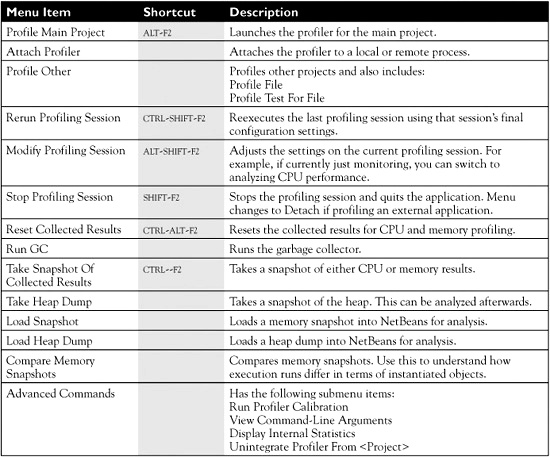
The first three menu items are used for initiating a profiling session. Profiling sessions are started for the current main project by invoking Profile | Profile Main Project or for other local and remote processes via Profile | Attach Profiler. The last option, Profile Other, has a submenu whose contents and status depend upon the active window. If the active window is an editor for a unit test, then menus for profiling the test or test suite appear under this menu. If the active window is Projects, the contents vary if a Java package is selected or a unit test or class with a main method is selected. Profiling options are also available when right-clicking a Java class or JUnit test in the Projects window.
The first option, Profile Main Project, profiles the current project. This option uses the current Run configuration in Project Properties. Profiling requires changes to the project build script and calibration of the project’s JVM. NetBeans detects whether these steps are necessary and prompts before changes are made.
The Attach Profiler menu option is used to profile an existing Java application. This application does not need to be a project in NetBeans nor do you need the source code for the application. You can profile any Java application—ranging from a NetBeans instance to GlassFish and IBM WebSphere. Attaching a profiler to an existing application is covered in the next section.
Before a project can be profiled, the JVM must be calibrated. Profiling involves adding instrumentation to the byte code of the profiled application. This instrumentation adversely imposes overhead, which must be factored out to collect accurate data. The calibrated data is JVM and machine configuration specific. If changes are made to a machine’s hardware configuration such as a faster hard drive or more random access memory (RAM), the JVM calibration should be regenerated. Regenerating calibration data is performed by choosing Profile | Advanced Commands | Run Profiler Calibration. The first time a profiling is performed, NetBeans automatically prompts to perform calibration.
Pay special attention to calibration on laptop computers. Modern laptops use dynamic frequency scaling to throttle the processor to conserve power and reduce heat output. Throttling the processor thus results in skewed data. Profiling an application must take into account the operating environment, and understanding settings outside of the profiler is imperative. Other applications running the computer can also affect profiling. For example, encoding a video while profiling changes the results.
Profiling code using System.currentTimeMillis() is not an accurate technique for collecting performance data. First, retrieving this time requires crossing the boundary from user space into protected space of the operating system. This results in a significant performance penalty. Nesting calls to System.currentTimeMillis() would thus skew the results. You can use DTrace on OpenSolaris/Solaris or Mac OS X to see the effect.
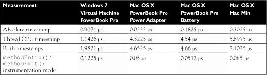
NetBeans displays the dialog box in Figure 10-13 the first time an application is profiled. After you click OK the calibration runs, and an option is presented to view the results. The results are shown in Figure 10-14. The results in Figure 10-14 are for a Windows 7 virtual machine running on a MacBook Pro using Parallels. For comparison, Table 10-5 lists a comparison between various machines. Differences are also shown for a laptop plugged into a power source and also running on battery.
FIGURE 10-13 VM calibration for profiling
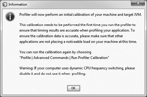
FIGURE 10-14 Calibration results
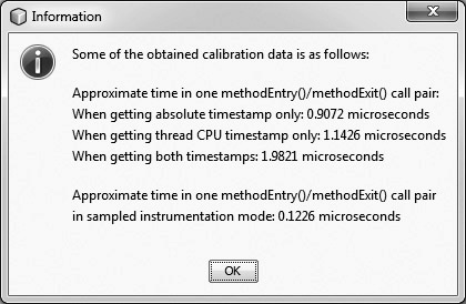
TABLE 10-5 Calibration Comparisons
Calibration data for the profiler is stored under .nbprofiler in a user’s home directory. This directory contains a binary with calibration data for each JVM that has been calibrated. The contents of this directory should not be shared across machines because profiling is machine specific.
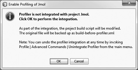
Profiling a project requires changes to the project’s Ant files. NetBeans warns before proceeding with the modifications. This dialog box is shown in Figure 10-15. NetBeans makes the following changes to the project:
FIGURE 10-15 Enabling profiling
![]() Create an nbproject/profiler-build-impl.xml script.
Create an nbproject/profiler-build-impl.xml script.
![]() Copy the current build.xml to build-before-profiler.xml script.
Copy the current build.xml to build-before-profiler.xml script.
![]() Create a new build.xml script.
Create a new build.xml script.
New files are scheduled for addition to version control. To revert these changes, choose Profiler | Advanced Commands | Unintegrate Profiler From <Application Name>. The only difference between the original build.xml created for a project and the profiler-specific instance is an import statement:
![]()
Attaching a Profiler to a Local Application
The second menu item in Table 10-4 is Attach Profiler. The NetBeans Profiler can be attached to both local and remote Java processes. The Java process being profiled does not need a corresponding project in NetBeans. This means that you can profile any Java application and even ones for which the source code is not available. Thus, if a particular project is not using NetBeans, the NetBeans Profiler can still be utilized. Having the project in NetBeans does bring benefits because it enables navigation from the profiler output to the source code. Attaching is also useful for profiling long-running applications or applications that have custom start scripts.
NetBeans supports three different attach modes. The attach mode chosen depends upon the location of the application, the JVM version being used, and the profiling statistics to be collected. The three modes include:
![]() Local Direct In this mode NetBeans launches the Java application so that profiling begins on startup. The application waits for NetBeans to connect to begin profiling.
Local Direct In this mode NetBeans launches the Java application so that profiling begins on startup. The application waits for NetBeans to connect to begin profiling.
![]() Local Dynamic In this mode the profiler can be attached to an application that is already running without restarting it. NetBeans and the application must be on the same computer. Java 6 or greater is required for this to work.
Local Dynamic In this mode the profiler can be attached to an application that is already running without restarting it. NetBeans and the application must be on the same computer. Java 6 or greater is required for this to work.
![]() Remote Direct In this mode applications running on a remote machine can be profiled. NetBeans generates a Remote Pack to be used in launching the application.
Remote Direct In this mode applications running on a remote machine can be profiled. NetBeans generates a Remote Pack to be used in launching the application.
![]()
The profiling exam objective does not require knowledge of remote profiling. Remote profiling involves connecting to a JVM running on a separate machine across the network. An example tutorial of profiling remote processes can be found at http://tinyurl.com/y4f3c2q.
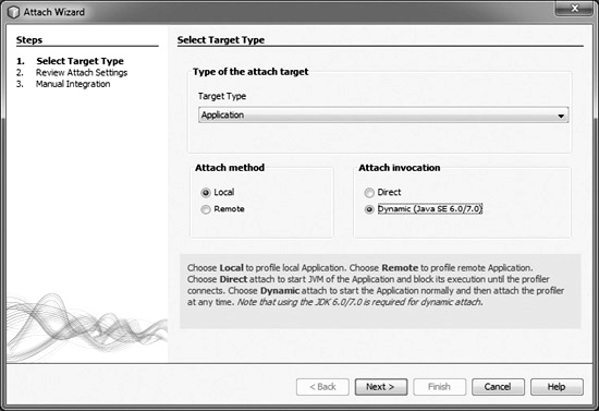
To attach to a JVM for profiling, choose Profile | Attach Profiler. This opens the dialog box shown in Figure 10-16. Clicking the Attach button opens the Attach Wizard shown in Figure 10-17. In this step we select the target type as well as the attachment method and invocation. As discussed previously, Dynamic enables the monitoring of applications that are already running, whereas Direct is used to monitor pre-Java 6 or situations where profiling should begin as soon as the application launches. Remote is not covered on the exam and thus is not discussed. NetBeans saves the choices made in Figure 10-17 for subsequent runs. To change the attach mode, the dialog box in Figure 10-16 includes a link for altering the configuration in place of the phrase “No attach settings defined.”
FIGURE 10-16 Attach external application
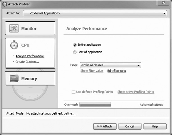
FIGURE 10-17 Attach Wizard: Select Target Type
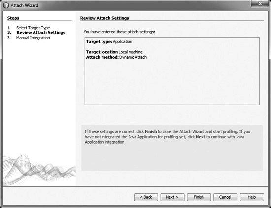
After you click Next, NetBeans displays a dialog box for reviewing the settings. An example is shown in Figure 10-18. The contents of this screen vary depending upon the target type.
FIGURE 10-18 Attach Wizard: Review Attach Settings
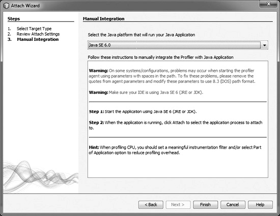
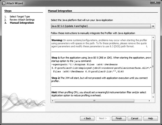
Clicking Next displays the Manual Integration step in the wizard, shown in Figure 10-19. This screen provides instructions and profiling advice. It also gives you a chance to launch the application and get it to the point where you want to begin profiling. Note, if the project is in NetBeans, you can set explicit profiling points.
FIGURE 10-19 Attach Wizard: Manual Integration
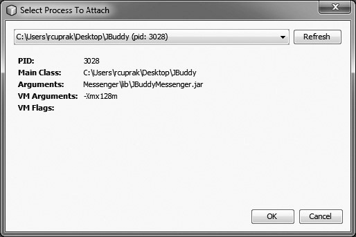
Once the application is launched, click Finish to display the dialog box shown in Figure 10-20. This dialog box has a drop-down list of the Java applications running on the computer along with their PID (process identifier). If you have multiple Java processes, you may need to use a platform-specific tool such as the Windows Task Manager to identify the process. Once OK is clicked, NetBeans attaches to the process and begins profiling it.
FIGURE 10-20 Select Process To Attach
When connecting to the local JVM for profiling, NetBeans opens a socket connection to the JVM. On Microsoft Windows a warning may appear: if you do not accept and allow NetBeans to open a connection, then you will not be able to profile.
Direct attachment is different. NetBeans provides command-line parameters that you must use to launch the application. These parameters vary depending upon the version of the JVM. Direct attachment is also the only way to connect to pre-Java 6 JVMs. Figure 10-21 shows the dialog box that is displayed after Figure 10-17 if Direct is chosen.
FIGURE 10-21 Attach Wizard: Manual Integration (direct)
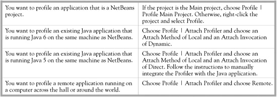
The Scenario & Solution helps you work through when to use each type of attachment mode for the profiler.
SCENARIO & SOLUTION
EXERCISE 10-4 Attaching the Profiler
In this exercise, you attach a profiler to an existing free commercial Java application. The source for this application is proprietary as well as obfuscated. This demonstrates the power of the NetBeans Profiler. Often you may have to use a profiler to understand how your application is affecting another Java application—for example, if you are using a commercial Java-based queuing system and it keeps running out of Java heap space while you are submitting messages. Java 6 is required for this exercise.
1. Download JBuddy Messenger from www.zionsoftware.com. JBuddy is a free Java-based instant-messaging client. It is a multithreaded Swing application.
2. Expand the downloaded JBuddy application and launch it. For the purposes of this exercise you do not need to log in to any AIM service.
3. In NetBeans, choose Profiler | Attach Profiler. If you have previously attached to another JVM, you need to click the change link for the attach mode; otherwise click Attach.
4. On the wizard panel for Select Target Type, make the following selections and click Next:
![]() Target Type: Application
Target Type: Application
![]() Attach Method: Local
Attach Method: Local
![]() Attach Invocation: Dynamic
Attach Invocation: Dynamic
5. On the Review Attach Settings wizard panel, click Finish.
6. In the dialog box for selecting the process, choose the drop-down entry for JBuddy and click OK.
7. The profiler now opens. To stop profiling, choose Profile | Detach. You have the option to either detach or terminate the application.
Monitoring a Desktop Application
The most basic type of profiling in NetBeans is monitoring. With monitoring, NetBeans uses no byte code instrumentation, and thus the impact of profiling is minimal. The information available is not much different than what is available through JConsole, a diagnostic tool included with the JDK. NetBeans uses information available through the Java Management Extension (JMX). Monitoring provides basic insight into an application including memory usage and thread activity. The data available is at a macroscopic level: how much heap space has been consumed and how it has changed over time, how many threads are running, and which threads are running or are in various nonrunning states. Monitoring is a relatively easy way to keep track of application behavior and to catch memory leaks while still in development.
Monitoring tracks and reports memory usage and thread usage over time. Three views are available for this type of monitoring:
![]() VM Telemetry Overview A window that contains three graphs summarizing application memory usage. This is the default view that is first opened.
VM Telemetry Overview A window that contains three graphs summarizing application memory usage. This is the default view that is first opened.
![]() VM Telemetry Opens a window with three tabs that provide a better view and tools for manipulating and exploring the graphs appearing in the VM Telemetry Overview window.
VM Telemetry Opens a window with three tabs that provide a better view and tools for manipulating and exploring the graphs appearing in the VM Telemetry Overview window.
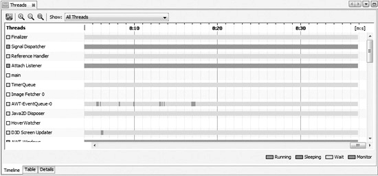
![]() Threads Opens a window with three tabs. Each tab displays a different view of the same thread data. The first tab includes a time, the second a table with the same data, and the third a pie chart.
Threads Opens a window with three tabs. Each tab displays a different view of the same thread data. The first tab includes a time, the second a table with the same data, and the third a pie chart.
Using monitoring, you can see and determine whether an application has a memory or thread leak. If an application has a memory leak, you see heap usage continue to increase over time. A thread leak manifests itself as a steady increase in threads over time. At any point during a profiling session the type of profiling data can be changed. If there appears to be a memory leak or problem with threading, you can choose Profile | Modify Profiling Session to change the data being collected.
Just because the heap continues to fill with objects doesn’t mean that you have a memory leak. A high-performance application may be using an object cache to reduce the performance penalty for frequent read operations that are I/O bound. An OutOfMemoryError can also mean that the garbage collector/heap settings haven’t been optimized for the application’s load.
Monitoring an application is split into the following subsections:
![]() Starting and Customizing Monitoring
Starting and Customizing Monitoring
![]() Understanding Telemetry Overview
Understanding Telemetry Overview
![]() Viewing Threads
Viewing Threads
Starting and Customizing Monitoring
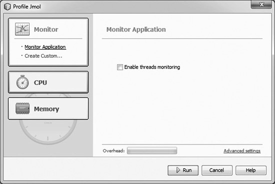
To monitor an application, choose any one of the first three actions under the Profile menu including Profile Main Project, Attach Profiler, or Profile Other. This displays a dialog box either the same or a similar to Figure 10-22. The boxes in the left panel—Monitor, CPU, and Memory—are actually buttons. Clicking the first button, Monitor, displays the basic monitor settings in the panel on the right. With basic settings, only one option is available, Enable Threads Monitoring. If this is checked, the NetBeans Profiler tracks threading performance from the moment the application starts. The Overhead bar toward the bottom of the dialog box graphically depicts the performance impact of this type of monitoring. Clicking Run in the dialog box launches the application and NetBeans begins profiling it.
FIGURE 10-22 Monitor Application
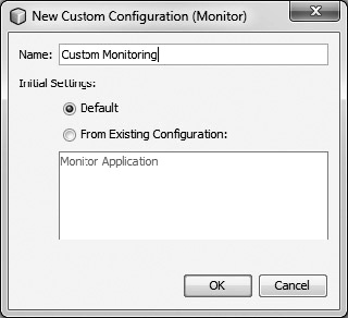
To edit the Advanced Settings, a custom monitoring configuration must be created. This is accomplished by clicking Create Custom under the Monitor button to display the dialog box in Figure 10-23. A custom configuration can be based upon either the default or another custom configuration.
FIGURE 10-23 New Custom Configuration
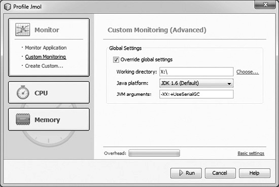
With a custom configuration in place, custom monitor parameters can be set, as shown in Figure 10-24. Custom parameters include Working Directory, Java Platform, and JVM Arguments. In this example the serial garbage collector has been specified to test its impact upon the performance of the application.
FIGURE 10-24 Custom monitoring configuration
Understanding Telemetry Overview
When the NetBeans Profiler launches in the monitoring mode, two new windows appear: Profiler at upper left and VM Telemetry Overview at lower right, as shown in Figure 10-25. (Placement may differ if you have previously used the profiler and rearranged your windows.)
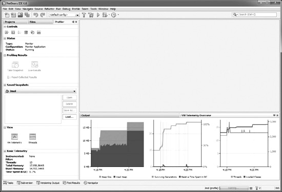
The VM Telemetry window is available regardless of the type of profiling being performed. If it does not appear automatically, it can be displayed via Window | Profiling | Profiling Telemetry Overview. It contains three graphs, each with the X axis representing time. Double-clicking a graph opens the graph in a larger window. The three graphs include:
![]() Memory Heap This graph displays the available heap versus the used heap. The initial heap size depends upon the initial heap (-Xmsn) and the minimum heap free ratio (-XX:MinHeapFreeRatio) The amount of heap continues to increase until it hits the maximum heap.
Memory Heap This graph displays the available heap versus the used heap. The initial heap size depends upon the initial heap (-Xmsn) and the minimum heap free ratio (-XX:MinHeapFreeRatio) The amount of heap continues to increase until it hits the maximum heap.
![]() Memory (GC) This graph shows two variables:
Memory (GC) This graph shows two variables:
![]() Relative Time Spent in GC This is the percentage of time spent in garbage collection. Scale is on the right.
Relative Time Spent in GC This is the percentage of time spent in garbage collection. Scale is on the right.
![]() Surviving Generations This is a number of generations currently on the heap. Scale is on the left.
Surviving Generations This is a number of generations currently on the heap. Scale is on the left.
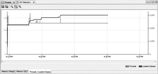
![]() Threads / Loaded Classes This graph shows two variables:
Threads / Loaded Classes This graph shows two variables:
![]() Threads Total number of threads in existence. Scale is on the right.
Threads Total number of threads in existence. Scale is on the right.
![]() Loaded Classes Total number of classes loaded into the JVM. Scale is on the left.
Loaded Classes Total number of classes loaded into the JVM. Scale is on the left.
Double-clicking a graph opens it in a larger window.
The Profiler control panel (window) on the left of Figure 10-25 manages the profiling session. It is organized into six panels that are the same regardless of the type of monitoring being performed. The six panels are:
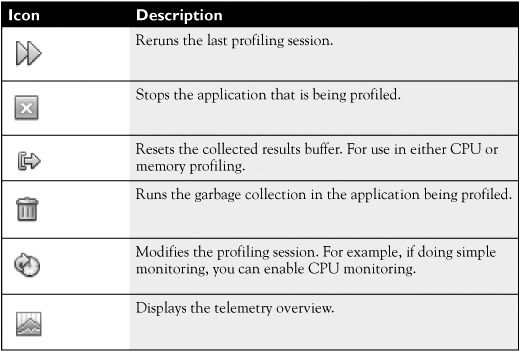
![]() Controls These controls are used to restart/stop the session as well as to change the parameters. The icons are documented in Table 10-6.
Controls These controls are used to restart/stop the session as well as to change the parameters. The icons are documented in Table 10-6.
![]() Status Displays the status of the session—specifically the type of monitoring being performed along with the name of the configuration.
Status Displays the status of the session—specifically the type of monitoring being performed along with the name of the configuration.
![]() Profiling Results Saves either a memory or CPU snapshot.
Profiling Results Saves either a memory or CPU snapshot.
![]() Saved Snapshots Lists saved CPU and memory snapshots. These snapshots can be reloaded into the editor for analysis and comparison.
Saved Snapshots Lists saved CPU and memory snapshots. These snapshots can be reloaded into the editor for analysis and comparison.
![]() View Displays either basic telemetry data, as shown in VM Telemetry Overview, or thread information.
View Displays either basic telemetry data, as shown in VM Telemetry Overview, or thread information.
![]() Basic Telemetry Displays basic information about the VM including the number of classes and threads as well as memory usage and a summary of the garbage collection.
Basic Telemetry Displays basic information about the VM including the number of classes and threads as well as memory usage and a summary of the garbage collection.
Selecting VM Telemetry from the View panel shown in Figure 10-25 opens a window with three tabs. These three tabs correspond to the three graphs on the VM Telemetry Overview window. The larger graphs, shown in Figures 10-26, 10-27, and 10-28, not only are easier to read, but they also track the entire history since profiling began. In addition, the mouse can be dragged over each graph to get a precise readout for any time point. Each of the three windows has a set of icons across the top for performing common actions. These are documented in Table 10-7.
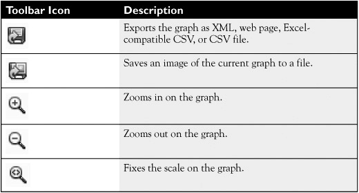
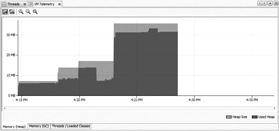
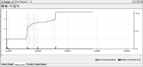
FIGURE 10-28 Threads/Loaded Classes
Viewing Threads
Thread telemetry data monitoring must be explicitly enabled. It can be enabled before profiling by choosing Enable Threads Monitoring shown in Figure 10-22. To view the threads, click the Threads icon in the View panel of the Profiler control panel shown in Figure 10-25. This opens a new editor window with the three tabs shown in Figures 10-29, 10-30, and 10-31. If thread monitoring was not enabled prior to running the application, NetBeans prompts for enabling it.
The first thread view, shown in Figure 10-29, is a graphical timeline of the application’s threads. Each thread is color-coded to show the state of the thread at a particular moment. The thread states are as follows:
![]() Running The thread is alive and performing tasks.
Running The thread is alive and performing tasks.
![]() Sleeping The thread is stopped on a Thread.sleep().
Sleeping The thread is stopped on a Thread.sleep().
![]() Wait The thread is stopped on a wait().
Wait The thread is stopped on a wait().
![]() Monitor The thread has stopped waiting to acquire a lock on a synchronized method.
Monitor The thread has stopped waiting to acquire a lock on a synchronized method.
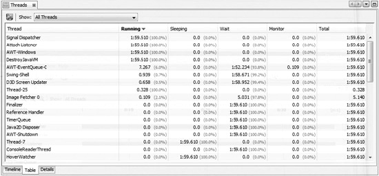
The second tab, shown in Figure 10-30, summarizes the information from Figure 10-29 in tabular form. In this view the percentage of time each thread spent in the different states is broken out. If an application has been running for a long time, this table provides a quick synopsis.
The Details tab, shown in Figure 10-31, combines the previous two tabs. In this view a color-coded pie chart is displayed along with the timeline for each thread. The threads being displayed can be filtered. An image snapshot can also be saved to disk.

The graphical view is useful if you are trying to understand what is going on in an application and how the execution of threads is being interleaved. If a deadlock is suspected, the debugging tools have the ability to detect deadlocks via Debug | Check For Deadlock.
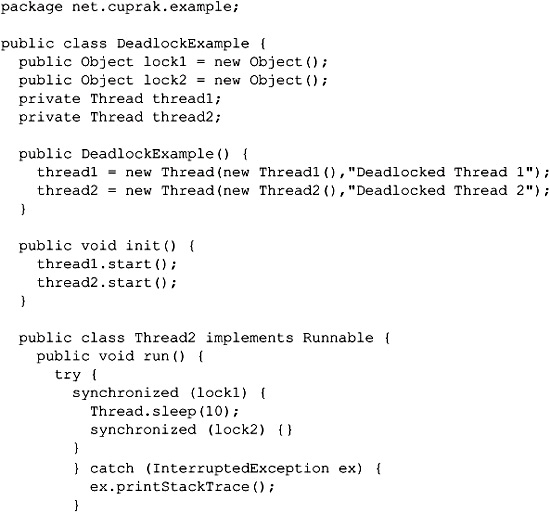
EXERCISE 10-5 Deadlocking Thread
In this exercise, you troubleshoot a deadlock. The following code creates a classic deadlock situation where each thread is attempting to acquire a lock. In the Threads view these two threads appear red, meaning that they are waiting for a monitor. You then use the debugger to verify the existence of a deadlock.
1. Create a new project by choosing File | New Project.
2. Select Java Application from the Java Category.
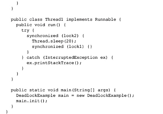
3. Pick a Project Name and specify the main class as net.cuprak.example.DeadlockExample.
4. Click Finish in the wizard, and replace the contents of the DeadlockExample.java file with:
5. Profile the project by either clicking the Profile toolbar icon or choosing Profile | Profile Main Project.
6. In the dialog box that appears (see Figure 10-22) select Monitor and then choose Enable Threads Monitoring.
7. Choose Run to begin profiling.
8. In the Profiler window, choose Threads under View.
9. Verify that “Deadlocked Thread 1” and “Deadlocked Thread 2” appear red and are thus deadlocked.
10. Stop the profiling session by choosing Stop from the Controls section of the Profiler window.
11. Choose Debug | Debug Main Project to start a debug session.
12. After the application has started, choose Debug | Check For Deadlock to verify the deadlock you saw in the Threads view.
Understanding CPU Performance
Analyzing performance involves tracking and understanding the amount of time spent in methods and constructors. To focus optimization activities, you need to know what specific parts of an application are consuming a disproportionate amount of CPU cycles. Without pinpointing the cause of performance problems, proposed solutions are merely conjecture that may only aggravate performance problems. The NetBeans Profiler collects and summarizes performance data, helping guide development planning.
This type of profiling is cumulative and can be reset. This means that at any given point you can clear the history and begin tracking method invocations from scratch. This enables you to determine how CPU resources were utilized between two points. For a file load operation, you would expect most of the time to be spent in I/O methods. To fully leverage this feature, you need profiling points that reset data collection and trigger snapshots. This section focuses on CPU performance profiling; the next section delves into profiler points.
The previous section discussed how to perform basic monitoring of an application. Those views, including VM Telemetry and Threads, are still available when profiling for performance and can be viewed at any time. Profiling an application for performance involves choosing the CPU group when initiating a profile session. When profiling starts, you have only two new views to worry about: Live Results and snapshot views.
Monitoring and collating CPU real-time performance data significantly derogates performance. For an interactive application such as Jmol that has been used in many exercises, the performance penalty is severe if not mitigated through planning and initial configuration of profiling parameters. NetBeans provides several mechanisms to control the scope of collected data including filters, profiling points, and sampling intervals. In addition, NetBeans can exclude code that will skew results such as invocations of sleep() and wait().
The following topics are covered:
![]() Configuring Performance Analysis
Configuring Performance Analysis
![]() Monitoring Performance
Monitoring Performance
![]() Capturing Snapshots
Capturing Snapshots
Configuring Performance Analysis
Initiating a performance profiling session is no different than initiating a monitoring session, as discussed in the previous section. When the Profile dialog box appears, select CPU, as shown in Figure 10-32. The basic settings are displayed by default. The following settings can be configured:
FIGURE 10-32 Profile: Analyze Performance
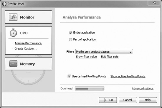
![]() Scope Either the entire application or just a portion of the application can be profiled. Limiting the scope improves performance. If Part Of Application is selected, a link appears next to it. The link displays a dialog box for selecting the methods to be profiled.
Scope Either the entire application or just a portion of the application can be profiled. Limiting the scope improves performance. If Part Of Application is selected, a link appears next to it. The link displays a dialog box for selecting the methods to be profiled.
![]() Filter Limits the classes that are to be profiled. The following choices can be made:
Filter Limits the classes that are to be profiled. The following choices can be made:
![]() Profile All Classes Profiles all classes in the application including external libraries.
Profile All Classes Profiles all classes in the application including external libraries.
![]() Profile Only Project Classes Profiles only classes that are a part of the project and are contained in the source directories. A link appears to display the options in this box shown in Figure 10-33.
Profile Only Project Classes Profiles only classes that are a part of the project and are contained in the source directories. A link appears to display the options in this box shown in Figure 10-33.
![]() Quick Filter Uses the pattern entered in the Set Quick Filter dialog box, as shown in Figure 10-34.
Quick Filter Uses the pattern entered in the Set Quick Filter dialog box, as shown in Figure 10-34.
![]() Exclude Java Core Classes Excludes core Java classes such as java.lang.String.
Exclude Java Core Classes Excludes core Java classes such as java.lang.String.
![]() Profiling Points If deselected, then custom profiling points are ignored.
Profiling Points If deselected, then custom profiling points are ignored.
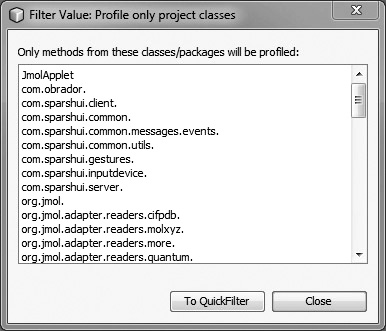
The profile filter dialog box shown in Figure 10-33 lists the project classes that are profiled when the filter is set to Profile Only Project Classes. Clicking the Show Filter Value link below the Filter drop-down list in Figure 10-32 opens the dialog box in Figure 10-33. The dialog box in Figure 10-33 is helpful for understanding what classes will be profiled. It is also helpful for bootstrapping a Quick Filter by choosing To QuickFilter. When this is done, the filter changes to Quick Filter, and the Set Quick Filter dialog box in Figure 10-34 appears. The Set Quick Filter dialog box is populated with classes from the project.
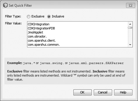
The Set Quick Filter dialog box, shown in Figure 10-34, is an editor that is used to quickly specify the classes that are to be profiled. Full package names must be used. The asterisk enables the specification of all classes within a package.
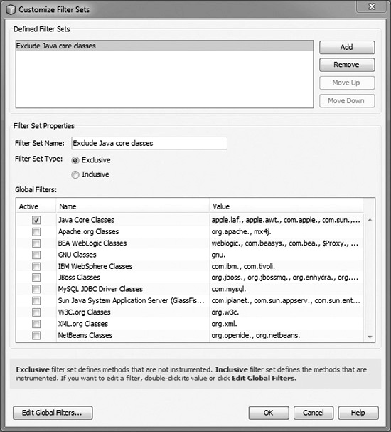
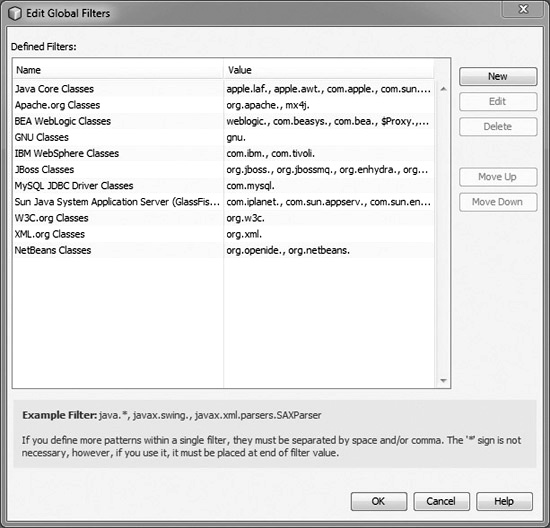
The filter sets available in the Filter drop-down list in Figure 10-32 are configured by clicking the link Edit Filter Sets below the list. This displays the dialog box shown in Figure 10-35. As can be seen from this screenshot, only the Java Core Classes are defined by default. New sets can be added. Each set makes use of a global library. The filter set can either include or exclude all of the classes in its global libraries. Global libraries are defined and edited by clicking Edit Global Filters.
FIGURE 10-35 Customize Filter Sets
The Edit Global Filters dialog box is shown in Figure 10-36. NetBeans includes numerous predefined libraries for common application servers and open source packages. Additional libraries can be added and then used in a custom filter set.
FIGURE 10-36 Edit Global Filters
Advanced configuration settings are configured by first creating a custom configuration by choosing Create Custom under CPU. After the custom configuration is created, choose Advanced Settings in the lower right of the dialog box, as shown in Figure 10-32. The custom settings then appear, as shown in Figure 10-37. The advanced settings are split into three categories: Settings, Threads, and Global Settings. The Settings category configures performance monitoring, whereas the last two categories are part of monitoring and were covered in the previous section. The following parameters are configured under Settings:
FIGURE 10-37 Advanced settings
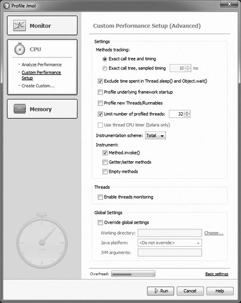
![]() Method Tracking You have two choices for this option: “Exact call tree timing” and “Exact call tree, sampled timing.” The first option records entry and exit time for each method every time. For the second option, method execution time is recorded only at specific intervals. The number of executions is still recorded.
Method Tracking You have two choices for this option: “Exact call tree timing” and “Exact call tree, sampled timing.” The first option records entry and exit time for each method every time. For the second option, method execution time is recorded only at specific intervals. The number of executions is still recorded.
![]() Exclude Time Spent in Thread.sleep() And Object.wait() Time spent in these methods would skew the results. However, if you are writing a multithreaded application, these can be very useful.
Exclude Time Spent in Thread.sleep() And Object.wait() Time spent in these methods would skew the results. However, if you are writing a multithreaded application, these can be very useful.
![]() Profile Underlying Framework Startup Profiles the startup of the JVM.
Profile Underlying Framework Startup Profiles the startup of the JVM.
![]() Profile New Threads/Runnables This setting is enabled when profiling an entire application. When the setting is selected, instrumentation is added to new threads.
Profile New Threads/Runnables This setting is enabled when profiling an entire application. When the setting is selected, instrumentation is added to new threads.
![]() Limit Number Of Profiled Threads Limits the number of profiled threads. Check the previous setting to profile all threads.
Limit Number Of Profiled Threads Limits the number of profiled threads. Check the previous setting to profile all threads.
![]() Instrumentation Scheme Instrumentation schemes determine the sequence in which methods are instrumented for profiling:
Instrumentation Scheme Instrumentation schemes determine the sequence in which methods are instrumented for profiling:
![]() Lazy This setting is best used when profiling only a part of the application. In Lazy, instrumentation isn’t performed until a root method is executed. Then all possible methods from this point are executed. This greatly reduces the scope of instrumentation as well as the performance impact.
Lazy This setting is best used when profiling only a part of the application. In Lazy, instrumentation isn’t performed until a root method is executed. Then all possible methods from this point are executed. This greatly reduces the scope of instrumentation as well as the performance impact.
![]() Eager This is a hybrid approach between Lazy and Total. It analyzes classes as soon as they are loaded for root methods and their dependencies.
Eager This is a hybrid approach between Lazy and Total. It analyzes classes as soon as they are loaded for root methods and their dependencies.
![]() Total This setting is used for profiling an entire application from the start. All of an application’s methods are instrumented as soon as they are loaded.
Total This setting is used for profiling an entire application from the start. All of an application’s methods are instrumented as soon as they are loaded.
![]() Instrument This setting is used to reduce the number of methods instrumented. Setter and getter methods don’t often affect performance, nor do empty methods.
Instrument This setting is used to reduce the number of methods instrumented. Setter and getter methods don’t often affect performance, nor do empty methods.
It is extremely important to understand these settings and how they impact performance. Adding instrumentation to a method is an expensive operation. Recording the execution time of a method is also very expensive. Elapsed time calculations require using the high-resolution timer specific to the operating system. If an application is call intensive—an interactive graphical application, for example—the impact is substantial and often renders the application barely usable. Minimizing the number of instrumented methods and data points significantly reduces the profiling overhead.
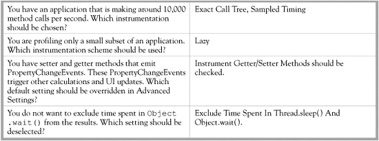
The Scenario & Solution helps you better understand these custom settings.
SCENARIO & SOLUTION
Monitoring Performance
Once the Run button is clicked in the Profile dialog box, shown in Figure 10-32, the NetBeans Profiler immediately launches the application. If the entire application is being profiled, data collection begins immediately. Otherwise the profiler waits until a profiler point is tripped. When profiling an application, the HotSpot virtual machine dynamically instruments the code. The just-in-time (JIT) compiler dynamically converts Java byte code to machine language. This means that an application being profiled should be “warm” before profiling results are collected.
To see the results while the application is running, click the Live Results icon in the Profiling Results panel of the Profile window. This opens the Live Profiling Results view shown in Figure 10-38. This window contains the following columns:
FIGURE 10-38 Live Profiling Results view

![]() Method Name of the method being invoked.
Method Name of the method being invoked.
![]() Self Time [%] Percentage of the runtime that the method consumed executing.
Self Time [%] Percentage of the runtime that the method consumed executing.
![]() Self Time Total amount of time the method has executed. Divide by the value in the Invocations column to get an average invocation time.
Self Time Total amount of time the method has executed. Divide by the value in the Invocations column to get an average invocation time.
![]() Invocations The number of times the method has been invoked.
Invocations The number of times the method has been invoked.
The icons appearing across the top of the table are documented in Table 10-8.
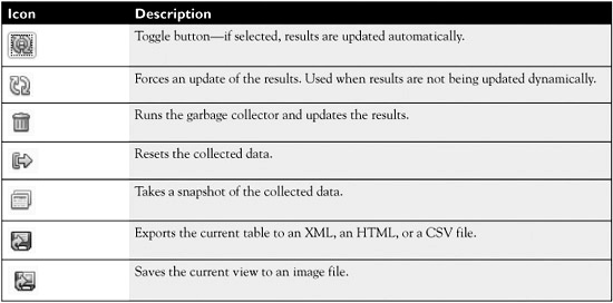
Capturing Snapshots
Snapshots of the profile data are captured by either clicking the icon in the Live Profiling Results window or by clicking the Take Snapshot button in Profiling Results. Additionally, choosing Profile | Take Snapshot Of Collected Results (CTRL-F2) also takes a snapshot. By default, a new snapshot window is created and shown in Figure 10-39. A snapshot window has four tabs:
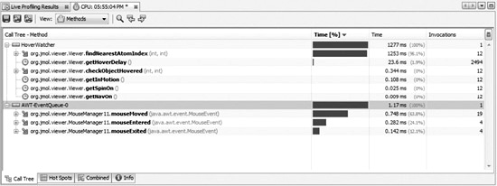
![]() Call Tree This tab displays the call tree for the method. The tree can be altered to show methods, classes, or packages.
Call Tree This tab displays the call tree for the method. The tree can be altered to show methods, classes, or packages.
![]() Hot Spots This tab is the same view of the data as shown in Figure 10-38.
Hot Spots This tab is the same view of the data as shown in Figure 10-38.
![]() Combined This tab combines the Call Tree and Hot Spots views into a split pane.
Combined This tab combines the Call Tree and Hot Spots views into a split pane.
![]() Info This tab summarizes configuration settings and root methods.
Info This tab summarizes configuration settings and root methods.
Right-clicking an entry in Figure 10-39 brings up a context menu with the following entries:
![]() Go To Source Opens entry in the Java source code file if source is available.
Go To Source Opens entry in the Java source code file if source is available.
![]() Show Subtree Shows the subtree for the selection.
Show Subtree Shows the subtree for the selection.
![]() Show Back Trace Shows the back trace for the current selection.
Show Back Trace Shows the back trace for the current selection.
![]() Find in Hot Spots Switches to the Hot Spots tab and highlights the selected method.
Find in Hot Spots Switches to the Hot Spots tab and highlights the selected method.
![]() Add To Instrumentation Roots Adds this method to the instrumentation roots. Instrumentation roots are used to winnow the list of methods being profiled. By using this action, you are adding an additional method to the set that is to trigger profiling.
Add To Instrumentation Roots Adds this method to the instrumentation roots. Instrumentation roots are used to winnow the list of methods being profiled. By using this action, you are adding an additional method to the set that is to trigger profiling.
A captured snapshot is not saved yet. To save the snapshot, click the toolbar icon for Save Snapshot To Project. The snapshot now appears in the Saved Snapshots of the Profile window.
![]()
The default behavior when taking a new snapshot is configured in Tools | Options | Miscellaneous | Profiler. Review these settings as you go through this chapter.
Using Profiling Points
Profiling points and root methods are an important feature of the NetBeans Profiler. They are used for both CPU and memory profiling. Conceptually they are very similar to debug breakpoints. When a particular line of code is executed in a debugger, you want to either pause execution to investigate application state or log a message to the console at the breakpoint. With profile points, you want to perform a specific action such as starting a timer, taking a snapshot, or initiating profiling. Profile points are invaluable for large applications where either the overhead of profiling would generate too much data, or the application would be unusable due to the overhead. The following topics will be covered:
![]() Understanding Profiling Point Basics
Understanding Profiling Point Basics
![]() Adding a Profile Root Method
Adding a Profile Root Method
![]() Selecting Multiple Root Methods
Selecting Multiple Root Methods
![]() Inserting a Profile Point
Inserting a Profile Point
Understanding Profiling Point Basics
Profile points are set in the code and are persisted between editing sessions like breakpoints. To add a profile point to code, you right-click within a Java source code file and choose one of the three options under Profile:
![]() Add As Profiling Root Method Adds a method as a root method. A root method triggers the profiler to begin collecting data.
Add As Profiling Root Method Adds a method as a root method. A root method triggers the profiler to begin collecting data.
![]() Select Profiling Root Methods Opens a dialog box for selecting multiple root methods within a class.
Select Profiling Root Methods Opens a dialog box for selecting multiple root methods within a class.
![]() Insert Profiling Point Inserts a new profile point.
Insert Profiling Point Inserts a new profile point.
When a profiling session is started that contains profiling points, the Profiling Points window opens, as shown in Figure 10-40. It lists the profiling points along with the project to which the points belong. If the profiling point has results, the results can be viewed by double-clicking the row. Profiling points can also be added, removed, and disabled. Note, profiling points cannot be added to the application while profiling is in progress.
FIGURE 10-40 Profiling Points window
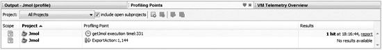
Adding a Profile Root Method
A profile root method triggers the profiler to begin collecting either CPU or memory data when any thread enters the method. All methods below the root method or objects created or destroyed are tracked. This is an easy way to limit profiling to a specific segment or module of an application. When right-clicking and choosing Profile | Add As Profiling Root Method, the cursor should be on a method. For example, in the following code listing you would right-click either testShowAboutBox or println:
public void testShowAboutBox() {
System.out.println("showAboutBox");
}
A dialog box then appears to prompt for the configuration the root method should be added to, as shown in Figure 10-41. Once a root method is set, the configuration switches over to being Part Of Application, as shown in Figure 10-32. A link appears next to the radio button for editing the list of root methods.
FIGURE 10-41 Select Settings Configuration
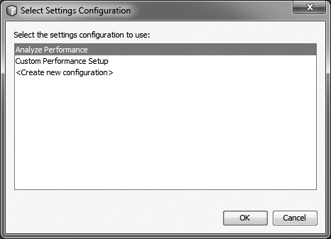
Selecting Multiple Root Methods
Choosing Select Profiling Root Methods enables you to select multiple root methods for a class. For example, if a class has 20 methods and you want to make 10 of them root methods, adding them individually would be a laborious process. For this menu item, you may click anywhere in a file. You are first prompted for the configuration to add your root methods to. Then a dialog box appears (example shown in Figure 10-42) for selecting the methods to be made into root methods.
FIGURE 10-42 Select Root Methods
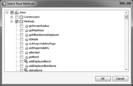
Inserting a Profile Point
Choosing Insert Profiling Point inserts a new profiling point into the code. This displays the dialog box shown in Figure 10-43. There are five different types of profile points listed next. Which profile point to select really depends upon the task at hand.
FIGURE 10-43 New Profiling Point
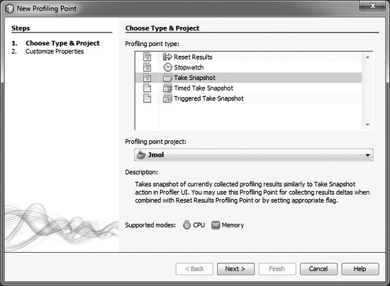
![]() Reset Results Resets the profiling results. This is often used to create diffs that can then be compared.
Reset Results Resets the profiling results. This is often used to create diffs that can then be compared.
![]() Stopwatch Used to output a timestamp and measure the time differences within a method fragment.
Stopwatch Used to output a timestamp and measure the time differences within a method fragment.
![]() Take Snapshot Takes a snapshot of the current collected results and then saves it for further analysis.
Take Snapshot Takes a snapshot of the current collected results and then saves it for further analysis.
![]() Timed Take Snapshot Takes a snapshot at a specific time. For example, this can be used to generate a snapshot if a batch process application fails every night in the middle of a run.
Timed Take Snapshot Takes a snapshot at a specific time. For example, this can be used to generate a snapshot if a batch process application fails every night in the middle of a run.
![]() Triggered Take Snapshot Takes a memory snapshot when a constraint such as available heap space, surviving generations, used heap space, or allocated heap reaches a specific threshold. Only available for memory snapshots.
Triggered Take Snapshot Takes a memory snapshot when a constraint such as available heap space, surviving generations, used heap space, or allocated heap reaches a specific threshold. Only available for memory snapshots.
Reset Results The Reset Results profiling point clears the statistics that have been collected. This is useful in combination with the Take Snapshot profile point, where the objective is to perform a diff. For example, place a Reset Results profile point in code before a file is loaded. After the file is loaded, use a Take Snapshot profile point to capture either memory or CPU statistics. You then know how many objects were created as a part of the open or where CPU resources were spent while loading. Figure 10-44 displays the configuration settings for a new Reset Results profile point. The settings include:
FIGURE 10-44 New Profiling Point: Reset Results
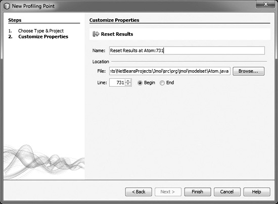
![]() Name Name of the profile point; includes the line number by default for readability.
Name Name of the profile point; includes the line number by default for readability.
![]() File The file in which the project point belongs.
File The file in which the project point belongs.
![]() Line Line number on which the profile point is to be set along with whether the action should be performed before or after the line executes.
Line Line number on which the profile point is to be set along with whether the action should be performed before or after the line executes.
Stopwatch The Stopwatch profile point enables the recording of a timestamp or the timing of a series of operations. The dialog box for creating a new Stopwatch profile point is shown in Figure 10-45. If Timestamp is selected when the Stopwatch profile point is tripped, the current time is recorded. If the Timestamp And Duration option is selected, then the start time and total execution time are recorded. The File and Line number for the profile point are also specified. The profile point can be executed either before the line executes or after it finishes. The end location is only enabled if the duration is being recorded. When you’re editing an existing Stopwatch profile point, a button to the right is displayed with the text “Current Line.” This button automatically populates the File and Line number boxes with the current cursor position. Stopwatch results are shown in Figure 10-46. Clicking the Report link shown in Figure 10-40 opens the results.
FIGURE 10-45 New Profiling Point: Stopwatch
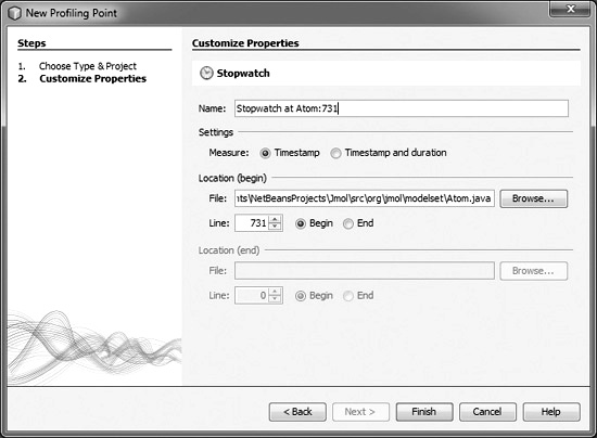
FIGURE 10-46 Stopwatch results
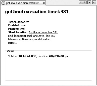
Take Snapshot The Take Snapshot profile point takes either a Profiling Data Snapshot or a Heap Dump. It is configured in the dialog box shown in Figure 10-47. A Profiling Data Snapshot is either a memory or thread snapshot depending upon the type of profiling being performed. Each time the profile point is triggered, a snapshot is generated. The snapshot can be saved either to the project or to a local directory. Optionally data collection can be reset after taking the snapshot.
FIGURE 10-47 New Profiling Point: Take Snapshot

Timed Take Snapshot A Timed Take Snapshot generates either a profile snapshot or a heap dump at a specific time or repeatedly with a time delay. It is configured using the dialog box shown in Figure 10-48. The type of profile snapshot generated depends upon whether CPU or memory monitoring is being performed. The snapshot or dump can either be saved to the project or to a local directory. Optionally, when the snapshot is taken, collected data can be reset. Unlike previous profile points, this one is not tied to a specific code location; instead it is triggered by an alarm. It can fire just once, or it can fire repeatedly at a predefined interval. This profile point lets long-running processes be monitored easily. For example, this could be used to track the performance of an application as it undergoes load testing over a period of several hours.
FIGURE 10-48 New Profiling Point: Timed Take Snapshot
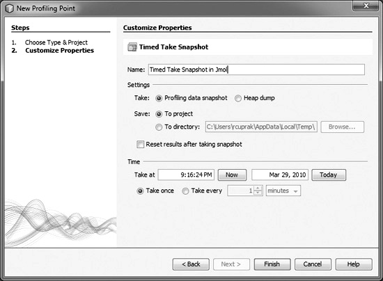
Triggered Take Snapshot A Triggered Take Snapshot, its configuration shown in Figure 10-49, is similar to a Time Take Snapshot. Like a Timed Take Snapshot it isn’t tied to a specific code location, and it also can generate either a CPU or memory snapshot, or a heap dump. It also can reset collected results. Where it differs is with the trigger that causes a snapshot or dump to be generated. A Triggered Take Snapshot can be initiated by one of the following conditions:
FIGURE 10-49 New Profiling Point:Triggered Take Snapshot
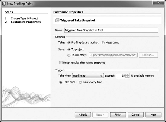
![]() Used heap exceeds a certain percentage of the total heap. For example, a snapshot could be generated when 98 percent of the heap has been consumed.
Used heap exceeds a certain percentage of the total heap. For example, a snapshot could be generated when 98 percent of the heap has been consumed.
![]() Allocated heap exceeds a predefined number of megabytes.
Allocated heap exceeds a predefined number of megabytes.
![]() Surviving generations exceed a specified number.
Surviving generations exceed a specified number.
![]() Loaded classes exceed a specified number.
Loaded classes exceed a specified number.
This profile point can be executed just once or each time the trigger condition is satisfied. It is useful for hard to replicate situations where you want the profiler to immediately capture data without requiring manual intervention.
Understanding Memory Usage
Memory profiling is a useful tool for understanding and exploring object creation and longevity. Creating an object and cleaning up after an object take time. When an object is created, space must be allocated on the heap and references tracked. When the object is no longer needed, the garbage collector must verify that the object is not reachable and compact memory to avoid fragmentation. Thus, needless object creation can have a significant impact upon performance that would not be visible from examining thread activity. This type of profiling seeks to answer:
![]() Between two points in time how many objects were created?
Between two points in time how many objects were created?
![]() What objects were created?
What objects were created?
![]() How long did the objects live?
How long did the objects live?
![]() How many of these objects were reachable at the end?
How many of these objects were reachable at the end?
![]() How many generations did the objects survive?
How many generations did the objects survive?
These questions can be answered by profiling memory use. The insight gained can then be used to optimize the code and reduce needless object creation. NetBeans facilitates this type of profiling. In addition, NetBeans can optionally track the creator of a class by capturing the stack trace. This is the Record Stack Trace For Allocations setting. This setting makes it possible to find who is instantiating the objects, which is extremely useful when tracking down memory leaks.
The following topics are covered in this section:
![]() Configuring for Memory Analysis
Configuring for Memory Analysis
![]() Capturing Snapshots
Capturing Snapshots
![]() Viewing Live Results
Viewing Live Results
![]() Comparing Allocations
Comparing Allocations
Configuring for Memory Analysis
Initiating a memory profiling session is done by choosing Profile | Profile Main Project or Profile | Attach Profiler. You can also initiate a session by clicking the menu item Profile | Profile Other or right-clicking a class with a main method or JUnit test and choosing Profile File. When the Profile dialog box appears, select Memory, as shown in Figure 10-50. The basic settings are displayed by default. The following settings can be configured:
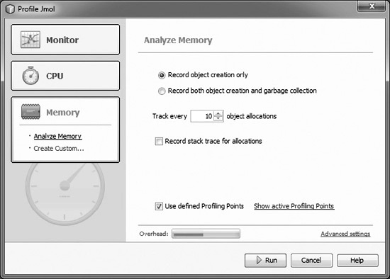
![]() Record Object Creation Only This setting causes the profiler to track the number of objects instantiated, their type, and bytes allocated.
Record Object Creation Only This setting causes the profiler to track the number of objects instantiated, their type, and bytes allocated.
![]() Record Both Object Creation And Garbage Collection This setting causes the profiler to track the number of objects instantiated, their type, bytes allocated, average age, generations, and objects that are live (reachable). Tracking this additional information significantly increases the overhead over the first option.
Record Both Object Creation And Garbage Collection This setting causes the profiler to track the number of objects instantiated, their type, bytes allocated, average age, generations, and objects that are live (reachable). Tracking this additional information significantly increases the overhead over the first option.
![]() Track Every n Object Allocations This option sets the interval/proportion for stack sampling. This controls the granularity of the data being collected. A value of 1 means that every object allocation is recorded, whereas a value of 10 means that every tenth object is captured. The lower the number the higher the overhead.
Track Every n Object Allocations This option sets the interval/proportion for stack sampling. This controls the granularity of the data being collected. A value of 1 means that every object allocation is recorded, whereas a value of 10 means that every tenth object is captured. The lower the number the higher the overhead.
![]() Record Stack Trace For Allocations This option causes the profiler to record the stack when an object is created. Using this, you can find out who is instantiating the objects.
Record Stack Trace For Allocations This option causes the profiler to record the stack when an object is created. Using this, you can find out who is instantiating the objects.
![]() Use Defined Profiling Points This enables the use of profiling points.
Use Defined Profiling Points This enables the use of profiling points.
These settings can have a dramatic impact upon the performance of the application. If a large application is being profiled, there are several ways to reduce the performance penalty:
![]() Set root methods so that you collect information only on problematic application parts.
Set root methods so that you collect information only on problematic application parts.
![]() Record only object creations.
Record only object creations.
![]() Set a reasonable allocation sampling value. A number too low with a long-running application can generate a tremendous amount of information.
Set a reasonable allocation sampling value. A number too low with a long-running application can generate a tremendous amount of information.
![]() Record stack traces only when necessary.
Record stack traces only when necessary.
The NetBeans Profiler can generate an overwhelming deluge of information. To focus the information generated, use profiling points and reset the collected data so that your analysis is targeted. Java applications generate thousands of objects, so a strategy is needed if the results are to be analyzed and correctly interpreted.
Additional advanced settings are available if a custom configuration is created. The advanced settings are shown in Figure 10-51. The parameters grouped under Settings pertain to memory profiling. The Threads and Global Settings parameters are discussed in the section on monitoring. The custom memory profiling settings are as follows:
FIGURE 10-51 Custom memory profile configuration
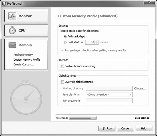
![]() Record Stack Trace For Allocations Either the full stack trace or just a subset of the stack trace can be recorded. For example, this is useful when working on a GUI application, because you don’t often care about the portion of the stack that invoked the menu item. Also, the more stack frames that are recorded, the bigger the impact upon performance.
Record Stack Trace For Allocations Either the full stack trace or just a subset of the stack trace can be recorded. For example, this is useful when working on a GUI application, because you don’t often care about the portion of the stack that invoked the menu item. Also, the more stack frames that are recorded, the bigger the impact upon performance.
![]() Run Garbage Collection When Getting Memory Results This setting gives you a better picture of what objects are actually live (reachable). This does result in a performance penalty.
Run Garbage Collection When Getting Memory Results This setting gives you a better picture of what objects are actually live (reachable). This does result in a performance penalty.
The first advanced setting is only enabled if stack traces are being collected.
Capturing Snapshots
Snapshots capture allocations made since the last reset. If there have been no resets, either from a profiling point or manually, then the allocation history extends to application startup. An allocation snapshot enables you to see the following:
![]() Class Name—Allocated Objects The type of the object instantiated. Double-clicking a row opens an editor for the class.
Class Name—Allocated Objects The type of the object instantiated. Double-clicking a row opens an editor for the class.
![]() Bytes Allocated Total number of bytes that the instances are consuming.
Bytes Allocated Total number of bytes that the instances are consuming.
![]() Objects Allocated Total number of objects instantiated. This includes objects that have been created and subsequently collected by the garbage collector.
Objects Allocated Total number of objects instantiated. This includes objects that have been created and subsequently collected by the garbage collector.
If garbage collection is included, that is, “Record both object creation and garbage collection,” the following additional statistics are collected:
![]() Live Bytes Total number of bytes that the live objects are consuming.
Live Bytes Total number of bytes that the live objects are consuming.
![]() Live Objects Total number of live objects that have not been garbage collected.
Live Objects Total number of live objects that have not been garbage collected.
![]() Avg. Age Average age of the objects in generations.
Avg. Age Average age of the objects in generations.
![]() Generations The number of different surviving generations that are currently alive on the heap.
Generations The number of different surviving generations that are currently alive on the heap.
Snapshots are captured either manually in NetBeans by clicking Take Snapshot in the Profiling Results group within the Profiler window or by a profiling point. A toolbar button is also present on Live Results for capturing snapshots. A snapshot opens in an editor tab with the timestamp prefixed with the word “Memory.” Snapshots created manually are not persisted until they are explicitly saved. An example snapshot is shown in Figure 10-52.
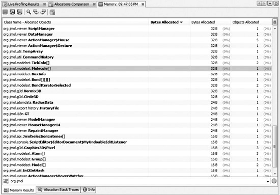
If stack traces are collected while profiling, right-clicking a class in Figure 10-52 and choosing Show Allocation Stack Traces opens the tab shown in Figure 10-53. The tab Allocation Stack Traces lists the different instances and where they were initially created. This is useful for determining who is creating the instances.
FIGURE 10-53 Memory: Allocation Stack Traces
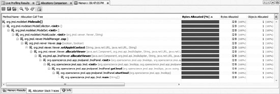
Results from Figures 10-52 and 10-53 can be exported for analysis in another application such as Microsoft Excel. A screenshot of the graph or table can be saved for inclusion in reports.
Viewing Live Results
While the application is running, the profiling data can be viewed live. Live Results are displayed by clicking the Live Results icon in the Profiling Results panel of the Profiler window. An example Live Profiling Results view is shown in Figure 10-54. As an application runs, the view dynamically changes. By default, the table is sorted with objects consuming the most heap space at the top. The columns are the same as for the memory snapshots. The available toolbar icons are the same as for the CPU profiling live results in Figure 10-38.
FIGURE 10-54 Live Profiling Results
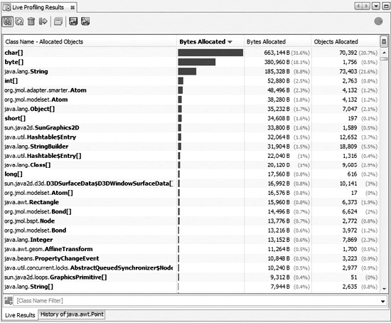
Right-clicking a class in Figure 10-54 and choosing Log Class History switches to the History tab, shown in Figure 10-55. In this view, we can track the number of objects instantiated for a particular class and the number of bytes they are consuming over time. Only one class can be viewed at a time.
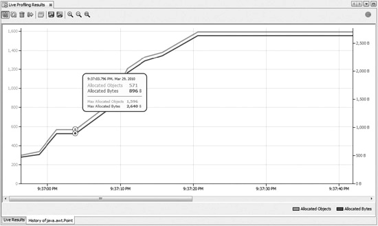
Comparing Allocations
One very handy feature of the NetBeans memory profiler is its ability to compare memory snapshots. Comparing memory snapshots enables you to quickly see what has changed. For example, you could take a snapshot before and after opening a file to see what objects were created. Or you could try two different algorithms for solving a particular problem, generate snapshots, and then compare them to see which one generated more or fewer objects.
Comparing memory snapshots is a powerful feature that can be used to track application memory performance over time. Before embarking on a refactoring job, a snapshot could be captured and then compared afterwards to evaluate the impact on memory utilization. This could also be done when new features are added.
An example memory comparison is shown in Figure 10-56. Here we can see the impact of opening a molecule in Jmol. Increases in objects created are shown as red bars that grow to the right. Decreases are represented as green bars that extend to the left. Profiles are compared by choosing Profile | Compare Memory Snapshots or by clicking the toolbar icon in a memory snapshot for performing a comparison. The memory snapshots compared do not have to be from the same JVM or even from the same application. For example, you could test the impact that upgrading to the latest JVM would have on memory use by comparing a snapshot running on one VM to another. This could also be done when evaluating app servers or other external libraries for inclusion in a project.
FIGURE 10-56 Allocations Comparison
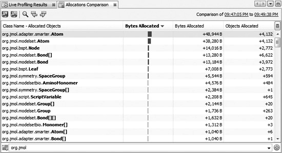
EXERCISE 10-6 Memory Profiling
In this exercise, you evaluate the memory footprints of using a java.util.LinkedList versus a java.util.ArrayList. Although the same number of objects is known ahead of time, we want to see the impact upon the heap of having to repeatedly resize an array.
1. Create a new Java project by choosing File | New Project and selecting Java Application from the Java category.
2. Change the contents of the main method to match this code:
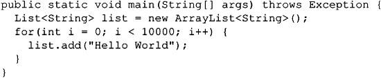
3. Profile the application by choosing Profile | Profile Main Project.
4. Choose Memory profiling.
5. Change object allocation tracking to 1.
6. Click Run to profile the application.
7. The application runs quickly and exits. NetBeans prompts you for saving the memory snapshot for the session. Accept and save the snapshot to the project.
8. Change the code so that you’re using a LinkedList instead of an ArrayList:
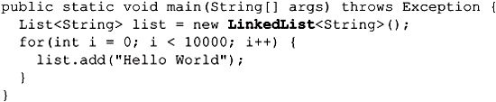
9. Profile the application again and save the snapshot to the project.
10. When a snapshot is taken, a tab is automatically opened in the IDE. With the last snapshot open, click the toolbar icon “Compare the difference between two comparable memory snapshots” to see the differences.
11. What’s different between these two runs?
12. For each memory snapshot, look over the list of objects created.
At the end of this exercise you may be puzzled by the results. Shouldn’t 10,000 Strings have been created? The JVM is quite intelligent, and it knows that the String class is immutable—hence only one instance is created. If you use another object such as a javax.swing.JFrame, you would see 10,000 javax.swing.JFrame instances. However, that still doesn’t explain the number of Strings created.
To better understand the number of Strings created, you can profile again and choose Record Stack Trace For Allocations to see where they are being instantiated. In the next section you learn how to inspect the content of the Strings.
Using the HeapWalker
The previous section covered memory profiling, which captures comprehensive statistics on the number of objects being created and destroyed as well as who instantiated them. The next question that naturally arises is how you find out what the objects contain. In Exercise 10-5, although we created just one String, the memory profile showed numerous instances.
What did the other instances contain? Knowing this bit of information can help trace memory leaks and get a better handle on the contents of the heap. This is where the heap analysis support in NetBeans comes into play.
The NetBeans Profiler can dump the contents of the Java heap to a file. Dumping the contents of a heap to a file is similar to creating a snapshot. In fact, all of the profile points support either generating a snapshot or a heap dump. A heap dump can also be manually generated by choosing Profile | Take Heap Dump. While a memory or CPU profile session is running, a toolbar icon is also present in the Live Results tab. Once the heap is captured, the NetBeans HeapWalker tool can be used for viewing and querying the heap.
Using the HeapWalker does not require that the application be profiled with NetBeans. The NetBeans HeapWalker reads in and analyzes heaps in the HPROF format. A heap dump created outside of NetBeans can be loaded into the HeapWalker by choosing Profile | Load Heap Dump. The following command line generates a heap dump for any running Java process:
![]()
The pid is the process identifier that is retrieved from the Task Manager in Windows or via the ps command on Unix-based systems. The jmap command-line application is included with the JDK. The command-line application jhat can also read the heap file and browse it.
To generate a heap dump, choose Profile | Take Heap Dump. This displays the dialog box shown in Figure 10-57. The heap dump can be saved either to the project or to a local directory. Heap dumps saved to the project appear under Saved Snapshots in the Profiler window.
FIGURE 10-57 Choose Heap Dump Destination
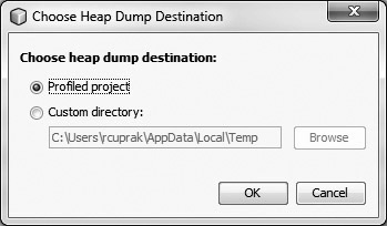
Once a heap dump is generated, NetBeans prompts for whether the heap dump should be opened in the HeapWalker. Opening the heap in the HeapWalker displays the window in Figure 10-58. This window is split into four tabs:
FIGURE 10-58 HeapWalker: Summary tab
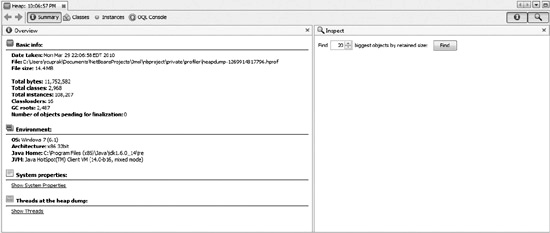
![]() Summary This tab displays basic summary information including:
Summary This tab displays basic summary information including:
![]() Basic JVM info
Basic JVM info
![]() Environment settings including the operating system and Java version
Environment settings including the operating system and Java version
![]() System properties
System properties
![]() Threads running at the time of the heap dump
Threads running at the time of the heap dump
![]() Classes This is a list of classes present on the heap. Double-clicking a class opens it on the Instances tab.
Classes This is a list of classes present on the heap. Double-clicking a class opens it on the Instances tab.
![]() Instances This is a list of instances of a class. You can browse the fields for each class, and see who is referencing them. This is useful for figuring out who is holding onto a reference and thus causing a memory leak.
Instances This is a list of instances of a class. You can browse the fields for each class, and see who is referencing them. This is useful for figuring out who is holding onto a reference and thus causing a memory leak.
![]() OQL Console This an interactive console for entering Object Query Language (OQL) queries. This enables you to search the heap using SQL-like expressions.
OQL Console This an interactive console for entering Object Query Language (OQL) queries. This enables you to search the heap using SQL-like expressions.
The first tab is shown in Figure 10-58. This tab summarizes the basic information about the JVM. On this tab you can find:
![]() Total number of classes.
Total number of classes.
![]() Total number of class instances contained in the file.
Total number of class instances contained in the file.
![]() Number of garbage collection roots.
Number of garbage collection roots.
![]() Version of the operating system.
Version of the operating system.
![]() Specific Java installation instance being used.
Specific Java installation instance being used.
![]() Specific Java version being used.
Specific Java version being used.
![]() A dump of system properties, which includes the classpath and parameters passed to the JVM among other things.
A dump of system properties, which includes the classpath and parameters passed to the JVM among other things.
![]() A dump of threads with their current points of execution. Line numbers are available if the code was compiled with debug symbols.
A dump of threads with their current points of execution. Line numbers are available if the code was compiled with debug symbols.
The second tab, shown in Figure 10-59, displays the list of classes that have been loaded. These are not class instances, but classes that were loaded by the JVM and subsequently instantiated or cached. This table includes some useful information including:
FIGURE 10-59 HeapWalker: Classes tab
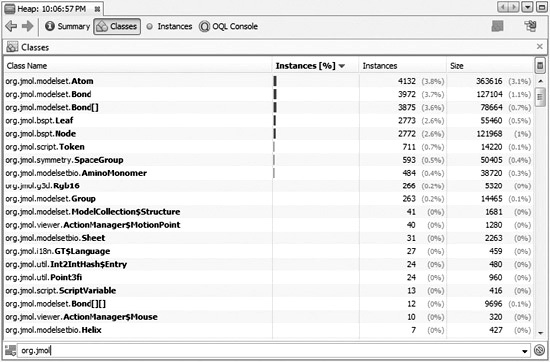
![]() Percent of the heap occupied by a class
Percent of the heap occupied by a class
![]() Number of instances created
Number of instances created
![]() Total space occupied by the instances
Total space occupied by the instances
Double-clicking a class in Figure 10-59 switches to the Instances tab shown in Figure 10-60. This tab is split up into three panels:
FIGURE 10-60 HeapWalker: Instances
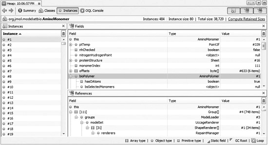
![]() Instances A list containing all of the instances of this object type in the heap.
Instances A list containing all of the instances of this object type in the heap.
![]() Fields Selecting an instance brings up a list of its fields that can be browsed. Double-clicking a field switches the view to that instance.
Fields Selecting an instance brings up a list of its fields that can be browsed. Double-clicking a field switches the view to that instance.
![]() References Using this view, you can see who is referencing this object. This is extremely useful when troubleshooting memory leaks.
References Using this view, you can see who is referencing this object. This is extremely useful when troubleshooting memory leaks.
On this tab you can browse specific instances and drill into them. You can see their instance variables and, most importantly, who is maintaining references to them. Knowing who is maintaining references is invaluable when trying to locate a memory leak. For example, you could see an object was still being stored in a java.util.List and then drill up to the owner of the list.
The fourth tab in the HeapWalker is the OQL Console, shown in Figure 10-61. This is one of the most exciting features of the HeapWalker. While the Instances tab is extremely useful, the amount of information can be overwhelming. A given application can have thousands of String instances. The challenge becomes sorting through all of these instances and finding the ones of interest.
FIGURE 10-61 HeapWalker: OQL Console
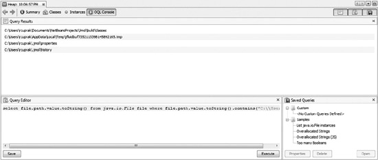
The HeapWalker’s OQL Console uses the Object Query Language. This language is modeled on SQL and developed by the Object Data Management Group. With this language, the contents of the heap can be filtered, sorted, and analyzed. OQL is also used by the jhat tool, which has similar functionality. Documentation OQL queries for jhat are applicable to NetBeans. A query has the following form:
![]()
The class name is a fully qualified name, for example, java.lang.String. The where expression is optional and uses JavaScript. The select expression evaluates JavaScript. NetBeans wraps up the Java heap objects in JavaScript objects. This means that values are accessed using dot notation. For example, to view the hash code of a String, the expression s.hash would be used. The s is a variable defined in the from clause—each Java object is bound to a variable. A query best illustrates this:
![]()
This query searches through the heap looking for String objects that contain “Hello World”. The toString() invocation is not the toString() method on the instance you are querying in the heap. It is a JavaScript toString() method. Also note the “==”, used for String comparison in JavaScript.
NetBeans OQL support also includes numerous built-in objects and functions that can be used in the queries. These objects and built-in functions provide a range of functionality enabling you to query for reachability, to filter, determine the size of objects, compare equality, and so on. The exam will not cover OQL in depth, and an entire book could be devoted to this language and how to effectively leverage it. Consult the online documentation in NetBeans by searching for “OQL.” The online documentation lists all of the built-in functions and objects and includes numerous examples.
The OQL queries are not against Java objects. Although the contents of Strings are being queried and you might see examples with methods that exist in Java, these methods are actually JavaScript methods. You cannot invoke String methods to perform evaluations when working with a heap dump. You are accessing the raw properties through a JavaScript wrapper instance. This means that if the property is computed, it isn’t available.
EXERCISE 10-7 Memory Profiling
In this exercise, you search through the Java heap for a particular String instance. This exercise builds on Exercise 10-5. In Exercise 10-5 we expected 10,000 String instances to be created. Memory profiling showed only 34 instances. We determine how many of the String instances contain “Hello World” and count how many instances refer to these instances.
1. Modify the code from Exercise 10-5 with the following addition:
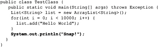
2. Select the line with System.out.println("Snap!"); and right-click, choosing Profiling | Insert Profiling Point.
3. Select Take Snapshot and click Next.
4. Select Heap Dump and click Finish.
5. Profile the project by choosing Profile | Profile Main Project.
6. Choose CPU profiling and click run.
7. The application launches and quits. A new heap dump is automatically captured.
8. Open the heap dump from the Saved Snapshots in the Profiler window.
9. Switch to the OQL Console tab.
10. Search for the “Hello World” String by performing the following search:
![]()
11. Notice that there was only one hit. Now issue the following query to determine how many classes refer to this instance:
![]()
12. Observe that “Hello World” was referred to 10,000 times.
13. To view who is referring to “Hello World”, issue the following query:
![]()
14. To view an entry, click it and the instance opens in the Instances tab.
In Exercise 10-5 the memory dump contained unexpected String instances. Issuing a query to count the number of String instances turns up considerably more this time. The previous memory snapshot did not include the myriad JVM Strings that are created by the JVM.
CERTIFICATION SUMMARY
This chapter covered JUnit integration and the NetBeans Profiler. Both of these features are invaluable tools for testing and verifying application behavior. JUnit is used for testing small granular units of application functionality to verify that that basic functionality works. JUnits form the basis of a regression suite to be executed regularly to confirm expected behavior. Profiling is used to explore the performance aspects of an application at runtime. Using a profiler, you can answer questions such as how many objects are being created, who is creating the objects, how long objects are living, as well as what the CPU and throughput bottlenecks are.
The first section of this chapter covered JUnit. JUnit topics covered included how to create new JUnit tests, run the JUnit tests, and view the results. Importantly, the different versions of JUnit supported by NetBeans were covered along with information on projects mixing versions. The last part of the section briefly discussed NetBeans’ Hudson integration, which enables unit tests to be run on a regular basis and monitored within the IDE.
The last half of this chapter covered the NetBeans Profiler. The NetBeans Profiler has three different modes: simple monitoring, CPU analysis, and memory analysis. NetBeans generates a calibration profile that is used to factor out the overhead of the profiler instrumentation. NetBeans can profile any Java application—either from a NetBeans project or running remotely on another machine. Monitoring provides basic telemetry information on the VM including heap usages, number of classes loaded, garbage collection impact, and thread activity. CPU analysis provides in-depth accounting of the time spent in methods. Memory analysis is used for tracking and understanding object creation and destruction. Memory snapshots can be generated, compared, and saved. In both CPU and memory profiling, profiling points can be used to trigger snapshots and reset results. The profiler also includes facilities for generating and reading heaps. A heap snapshot can be loaded into the HeapWalker, and the contents of the heap can be either browsed or searched using OQL.
 TWO-MINUTE DRILL
Testing Applications with JUnit
![]() NetBeans supports JUnit 3.x and JUnit 4.x.
NetBeans supports JUnit 3.x and JUnit 4.x.
![]() NetBeans prompts on the first unit test being created for the JUnit version.
NetBeans prompts on the first unit test being created for the JUnit version.
![]() NetBeans automatically adds either JUnit 3.x or JUnit 4.x libraries to the classpath.
NetBeans automatically adds either JUnit 3.x or JUnit 4.x libraries to the classpath.
![]() JUnit 4.x requires Java SE 5 or greater.
JUnit 4.x requires Java SE 5 or greater.
![]() JUnit 4.x makes extensive use of annotations.
JUnit 4.x makes extensive use of annotations.
![]() JUnit 3 and JUnit 4 conventions cannot be mixed in the same unit test case.
JUnit 3 and JUnit 4 conventions cannot be mixed in the same unit test case.
![]() Empty JUnit tests are created by choosing File | New File and selecting JUnit Test from the JUnit category.
Empty JUnit tests are created by choosing File | New File and selecting JUnit Test from the JUnit category.
![]() A JUnit for an existing class can be created by choosing File | New File and selecting Test For Existing Class from the JUnit category.
A JUnit for an existing class can be created by choosing File | New File and selecting Test For Existing Class from the JUnit category.
![]() A test suite for an existing class can be created by choosing File | New File and selecting Test Suite.
A test suite for an existing class can be created by choosing File | New File and selecting Test Suite.
![]() JUnit test classes are placed in a test sources directory.
JUnit test classes are placed in a test sources directory.
![]() A different classpath is used for unit test compiling and running unit tests.
A different classpath is used for unit test compiling and running unit tests.
![]() The unit testing classpath is configured in Project Properties on the Compile Tests and Run Tests tabs of the Libraries category.
The unit testing classpath is configured in Project Properties on the Compile Tests and Run Tests tabs of the Libraries category.
Using the NetBeans Profiler
![]() NetBeans includes a built-in profiler.
NetBeans includes a built-in profiler.
![]() The profiler measures the performance of a Java application in terms of memory use and threading.
The profiler measures the performance of a Java application in terms of memory use and threading.
![]() A NetBeans project is not required to profile a Java application.
A NetBeans project is not required to profile a Java application.
![]() Applications to be profiled can be either local or remote.
Applications to be profiled can be either local or remote.
![]() Applications to be profiled can be started outside of NetBeans.
Applications to be profiled can be started outside of NetBeans.
![]() The NetBeans Profiler has its own dedicated menu.
The NetBeans Profiler has its own dedicated menu.
![]() Profile operations are launched either from the toolbar, by right-clicking a JUnit test or class with a main method, or from the first three options in the Profile menu.
Profile operations are launched either from the toolbar, by right-clicking a JUnit test or class with a main method, or from the first three options in the Profile menu.
![]() To launch the profiler on the current main project, choose Profile | Profile Main Project.
To launch the profiler on the current main project, choose Profile | Profile Main Project.
![]() To attach a profiler to a running application, choose Profile | Attach Profiler.
To attach a profiler to a running application, choose Profile | Attach Profiler.
![]() Calibration is done before running the profiler for the first time.
Calibration is done before running the profiler for the first time.
![]() Calibration should be performed whenever there is a configuration change to a machine.
Calibration should be performed whenever there is a configuration change to a machine.
![]() Calibration and profiling are affected by low power consumption modes on laptops.
Calibration and profiling are affected by low power consumption modes on laptops.
![]() Profiling is controlled from the Profiler window in NetBeans.
Profiling is controlled from the Profiler window in NetBeans.
![]() The Profiler window is divided into six sections: Controls, Status, Profiling Results, Saved Snapshots, View, and Basic Telemetry.
The Profiler window is divided into six sections: Controls, Status, Profiling Results, Saved Snapshots, View, and Basic Telemetry.
![]() Windows related to the profiler can be reopened from Window | Profiler.
Windows related to the profiler can be reopened from Window | Profiler.
![]() There are three profiling modes: Monitor, Analyze CPU, Analyze Memory.
There are three profiling modes: Monitor, Analyze CPU, Analyze Memory.
![]() Monitor mode displays basic VM telemetry information including thread state, memory utilization, and garbage collection.
Monitor mode displays basic VM telemetry information including thread state, memory utilization, and garbage collection.
![]() Telemetry data collected in the monitor mode is available in all the other profiling modes.
Telemetry data collected in the monitor mode is available in all the other profiling modes.
![]() CPU and memory profiling are mutually exclusive.
CPU and memory profiling are mutually exclusive.
![]() CPU monitoring tracks the amount of time spent in methods and constructors.
CPU monitoring tracks the amount of time spent in methods and constructors.
![]() Methods profiled can be filtered to reduce the overhead and to target specific blocks of code.
Methods profiled can be filtered to reduce the overhead and to target specific blocks of code.
![]() Time spent in Thread.sleep and Object.wait() can be excluded from profiled results.
Time spent in Thread.sleep and Object.wait() can be excluded from profiled results.
![]() The number of threads profiled can be limited.
The number of threads profiled can be limited.
![]() There are two types of method tracking: “Exact call tree timing” and “Exact call tree, sampled timing.”
There are two types of method tracking: “Exact call tree timing” and “Exact call tree, sampled timing.”
![]() The three instrumentation schemes are Lazy, Eager, and Total.
The three instrumentation schemes are Lazy, Eager, and Total.
![]() Live Results displays collected statistics in real time.
Live Results displays collected statistics in real time.
![]() The following profile points are supported: Reset Results, Stopwatch, Take Snapshot, Timed Take Snapshot, Triggered Take Snapshots.
The following profile points are supported: Reset Results, Stopwatch, Take Snapshot, Timed Take Snapshot, Triggered Take Snapshots.
![]() The Reset Results profile point clears either CPU or memory profile data.
The Reset Results profile point clears either CPU or memory profile data.
![]() The Stopwatch profile point can either print a timestamp or compute the elapsed time between two execution points.
The Stopwatch profile point can either print a timestamp or compute the elapsed time between two execution points.
![]() Take Snapshot can capture CPU, memory, or heap snapshots when a specific line of code is executed.
Take Snapshot can capture CPU, memory, or heap snapshots when a specific line of code is executed.
![]() Timed Take Snapshot captures a CPU, memory, or heap snapshot at either a specific time or repeatedly with a delay.
Timed Take Snapshot captures a CPU, memory, or heap snapshot at either a specific time or repeatedly with a delay.
![]() Triggered Snapshot takes a snapshot when a particular event occurs such as a certain percentage of heap is exceeded.
Triggered Snapshot takes a snapshot when a particular event occurs such as a certain percentage of heap is exceeded.
![]() Memory snapshots can capture object creation, object destruction, and/or the stack trace at creation.
Memory snapshots can capture object creation, object destruction, and/or the stack trace at creation.
![]() Memory snapshots include data on the class name, bytes allocated, and objects allocated.
Memory snapshots include data on the class name, bytes allocated, and objects allocated.
![]() If memory profiling includes object destruction, then live bytes, live objects, average age, and generations will also be tracked.
If memory profiling includes object destruction, then live bytes, live objects, average age, and generations will also be tracked.
![]() Memory profiling results can be viewed during runtime by clicking Live Results in the Profiler window.
Memory profiling results can be viewed during runtime by clicking Live Results in the Profiler window.
![]() Right-clicking and choosing Log Class History from the context menu can track the history of an individual class.
Right-clicking and choosing Log Class History from the context menu can track the history of an individual class.
![]() Memory snapshots can be compared by choosing Profile | Compare Memory Snapshots.
Memory snapshots can be compared by choosing Profile | Compare Memory Snapshots.
![]() The HeapWalker provides a UI for viewing heap dumps.
The HeapWalker provides a UI for viewing heap dumps.
![]() Choosing Profile | Take Heap Dump or using a toolbar icon in the Live Results window generates a heap dump.
Choosing Profile | Take Heap Dump or using a toolbar icon in the Live Results window generates a heap dump.
![]() A heap dump can be generated while profiling for CPU or memory statistics.
A heap dump can be generated while profiling for CPU or memory statistics.
![]() Heap dumps are generated in the HPROF format.
Heap dumps are generated in the HPROF format.
![]() The HeapWalker can read heap dumps generated by jmap.
The HeapWalker can read heap dumps generated by jmap.
![]() The HeapWalker has four tabs: Summary, Classes, Instances, OQL Console.
The HeapWalker has four tabs: Summary, Classes, Instances, OQL Console.
![]() The Summary tab displays summary information including the JVM version and platform.
The Summary tab displays summary information including the JVM version and platform.
![]() The Classes tab displays the list of the classes that have been loaded by the JVM.
The Classes tab displays the list of the classes that have been loaded by the JVM.
![]() Double-clicking a class in the Classes tab switches to the Instances tab.
Double-clicking a class in the Classes tab switches to the Instances tab.
![]() The Instances tab displays all instances of a particular class.
The Instances tab displays all instances of a particular class.
![]() The Instances tab lists the classes referencing the instance.
The Instances tab lists the classes referencing the instance.
![]() The OQL Console tab displays a console for entering OQL queries for searching the Java heap. OQL is a SQL-like query language.
The OQL Console tab displays a console for entering OQL queries for searching the Java heap. OQL is a SQL-like query language.
![]() OQL is an acronym for the Object Query Language.
OQL is an acronym for the Object Query Language.
![]() OQL queries use JavaScript expressions.
OQL queries use JavaScript expressions.
![]() OQL support includes many functions including functions for reachability.
OQL support includes many functions including functions for reachability.
SELF TEST
The following questions will help you measure your understanding of the material presented in this chapter. Read all the choices carefully because there might be more than one correct answer. Choose all correct answers for each question.
Testing Applications with JUnit
1. What key shortcut will test the main project?
A. CTRL-N
B. CTRL-M
C. ALT-F6
D. F8
2. When does NetBeans prompt for the version of JUnit to be used for a project?
A. After the first JUnit is added to a project.
B. When the project is initially created.
C. NetBeans does not prompt; it is automatically set to the most recent version included with the IDE.
D. JUnit must be manually added to the classpath.
3. You would like to generate JUnit test classes for each class in a package. You would also like to generate a test suite for all of the tests. How would you go about doing this?
A. Select the package containing the classes in the Projects window and press CTRL-SHIFT-U.
B. Select the package containing the classes in the Projects window and right-click, choosing Tools | Create JUnit Tests.
C. Both A and B.
D. JUnit tests and test suites must be created individually for each class.
4. Which icon glyph is added to a JUnit test method that fails?
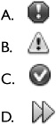
5. How can an individual unit test method be executed or debugged?
A. Individual test methods cannot be executed or debugged.
B. Individual test methods can be executed by performing a right-click in the Navigator window on the method and choosing Debug Test or Run Test.
C. Right-click the method name in the editor, and choose Debug or Run Test.
D. Right-click the method in the Test Results window and choose Run Again.
6. NetBeans supports which continuous integration server?
A. Apache Continuum
B. Apache Gump
C. CruiseControl
D. Hudson
Using the NetBeans Profiler
7. A project has been experiencing performance problems in a production environment requiring regular restarts. To troubleshoot the problem, you open the project in NetBeans to profile it. How do you launch the profiler and application from within NetBeans?
A. Debug | Profile Main Project
B. Profile | Profile Main Project
C. Profile | Attach Profiler
D. Tools | Profiler Tools
8. A computer that is regularly used for profiling undergoes a major operating system upgrade. What must be done to ensure accurate profiling?
A. NetBeans must be updated to the latest version.
B. The JDK must be reinstalled.
C. The profiler must be calibrated using Profile | Advanced Commands | Run Profiler Calibration.
D. Nothing needs to be done.
9. Which file is not changed or added when profiling?
A. nbproject/build-impl.xml
B. nbproject/profiler-build-mpl.xml
C. build.xml
D. build-before-profiler.xml
10. True or False? CPU and memory snapshots can be captured concurrently in the same profiling sessions.
A. True
B. False
11. You have created a custom configuration for CPU performance profiling. You will only be profiling a small subset of the application. What is the optimal instrumentation scheme?
A. Lazy
B. Eager
C. Total
D. Aggressive
12. Which icon represents a profiling point in the code?
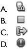
13. Which of the following is a valid OQL expression?
A. select s from java.lang.String s where s.equals("You Rule!")
B. select s from String s where s = 'You Rule!'
C. select * from java.lang.String s
D. select s from java.lang.String s where s.toString() == "You rule!"
SELF TEST ANSWERS
Testing Applications with JUnit
1. What key shortcut will test the main project?
A. CTRL-N
B. CTRL-M
C. ALT-F6
D. F8
![]() C. The key shortcut ALT-F6 will run the JUnits in the main project.
C. The key shortcut ALT-F6 will run the JUnits in the main project.
![]() A, B, and D are incorrect. A is incorrect because CTRL-N opens the New File Wizard. B is incorrect because CTRL-M performs the Move refactoring action. D is incorrect because F8 steps over code in the debugger.
A, B, and D are incorrect. A is incorrect because CTRL-N opens the New File Wizard. B is incorrect because CTRL-M performs the Move refactoring action. D is incorrect because F8 steps over code in the debugger.
2. When does NetBeans prompt for the version of JUnit to be used for a project?
A. After the first JUnit is added to a project.
B. When the project is initially created.
C. NetBeans does not prompt; it is automatically set to the most recent version included with the IDE.
D. JUnit must be manually added to the classpath.
![]() A. NetBeans prompts for the JUnit version to be used for a project after the first JUnit is added to the project.
A. NetBeans prompts for the JUnit version to be used for a project after the first JUnit is added to the project.
![]() B, C, and D are incorrect. B is incorrect because NetBeans does not prompt for the JUnit version when it first creates a project. C is incorrect because NetBeans makes no assumptions about the version of JUnit to be used. D is incorrect because NetBeans will add JUnit to the classpath when you create the first unit test.
B, C, and D are incorrect. B is incorrect because NetBeans does not prompt for the JUnit version when it first creates a project. C is incorrect because NetBeans makes no assumptions about the version of JUnit to be used. D is incorrect because NetBeans will add JUnit to the classpath when you create the first unit test.
3. You would like to generate JUnit test classes for each class in a package. You would also like to generate a test suite for all of the tests. How would you go about doing this?
A. Select the package containing the classes in the Projects window and press CTRL-SHIFT-U.
B. Select the package containing the classes in the Projects window and right-click, choosing Tools | Create JUnit Tests.
C. Both A and B.
D. JUnit tests and test suites must be created individually for each class.
![]() C. Both CTRL-SHIFT-U and Tools | Create JUnit Tests on the context menu will create both unit tests and a test suite for a package when a package node is selected in the Projects window.
C. Both CTRL-SHIFT-U and Tools | Create JUnit Tests on the context menu will create both unit tests and a test suite for a package when a package node is selected in the Projects window.
![]() A, B, and D are incorrect. A is incorrect because the context menu option Tools | Create JUnit Tests will also work. B is incorrect because CTRL-SHIFT-U is also correct. D is incorrect because unit tests and a test suite can be created for a project by selecting the project and choosing CTRL-SHIFT-U or by right-clicking and choosing Tools | Create JUnit Tests.
A, B, and D are incorrect. A is incorrect because the context menu option Tools | Create JUnit Tests will also work. B is incorrect because CTRL-SHIFT-U is also correct. D is incorrect because unit tests and a test suite can be created for a project by selecting the project and choosing CTRL-SHIFT-U or by right-clicking and choosing Tools | Create JUnit Tests.
4. Which icon glyph is added to a JUnit test method that fails?
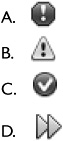
![]() B. This badge is displayed on unit tests that have failed.
B. This badge is displayed on unit tests that have failed.
![]() A, C, and D are incorrect. A is incorrect because that icon appears on a unit test, not the individual test methods that have failed. C is incorrect because that badge appears on unit tests that have succeeded. D is incorrect because that icon is clicked to rerun unit tests.
A, C, and D are incorrect. A is incorrect because that icon appears on a unit test, not the individual test methods that have failed. C is incorrect because that badge appears on unit tests that have succeeded. D is incorrect because that icon is clicked to rerun unit tests.
5. How can an individual unit method be executed or debugged?
A. Individual test methods cannot be executed or debugged.
B. Individual test methods can be executed by performing a right-click in the Navigator window on the method and choosing Debug Test or Run Test.
C. Right-click the method name in the editor, and choose Debug or Run Test.
D. Right-click the method in the Test Results window and choose Run Again.
![]() D. Individual unit test methods can only be run once all of the unit tests for a project have been executed. To run an individual unit test method, right-click the test on the method in the Test Results window and choose Run Again.
D. Individual unit test methods can only be run once all of the unit tests for a project have been executed. To run an individual unit test method, right-click the test on the method in the Test Results window and choose Run Again.
![]() A, B, and C are incorrect. A is incorrect because individual JUnit test methods can be run only after all of the unit tests for that JUnit class have been executed. B is incorrect because individual unit test methods cannot be executed from the Navigator window. C is incorrect because there is no context-specific menu in the Editor window for methods.
A, B, and C are incorrect. A is incorrect because individual JUnit test methods can be run only after all of the unit tests for that JUnit class have been executed. B is incorrect because individual unit test methods cannot be executed from the Navigator window. C is incorrect because there is no context-specific menu in the Editor window for methods.
6. NetBeans supports which continuous integration server?
A. Apache Continuum
B. Apache Gump
C. CruiseControl
D. Hudson
![]() D. NetBeans supports the Hudson continuous integration server.
D. NetBeans supports the Hudson continuous integration server.
![]() A, B, and C are incorrect. A is incorrect because NetBeans does not support Apache Continuum. B is incorrect because NetBeans does not support Apache Gump. C is incorrect because NetBeans does not support CruiseControl.
A, B, and C are incorrect. A is incorrect because NetBeans does not support Apache Continuum. B is incorrect because NetBeans does not support Apache Gump. C is incorrect because NetBeans does not support CruiseControl.
Using the NetBeans Profiler
7. A project has been experiencing performance problems in a production environment requiring regular restarts. To troubleshoot the problem, you open the project in NetBeans to profile it. How do you launch the profiler and application from within NetBeans?
A. Debug | Profile Main Project
B. Profile | Profile Main Project
C. Profile | Attach Profiler
D. Tools | Profiler Tools
![]() B. The NetBeans Profiler for the main project is launched using Profile | Profile Main Project.
B. The NetBeans Profiler for the main project is launched using Profile | Profile Main Project.
![]() A, C, and D are incorrect. A is incorrect because Profile Main Project does not appear in the Debug menu. C is incorrect because Attach Profiler is used to attach the profiler to a local or remote application that is not launched by NetBeans. D is incorrect because Profiler Tools is used to configure profiling for profiling native C++ applications.
A, C, and D are incorrect. A is incorrect because Profile Main Project does not appear in the Debug menu. C is incorrect because Attach Profiler is used to attach the profiler to a local or remote application that is not launched by NetBeans. D is incorrect because Profiler Tools is used to configure profiling for profiling native C++ applications.
8. A computer that is regularly used for profiling undergoes a major operating system upgrade. What must be done to ensure accurate profiling?
A. NetBeans must be updated to the latest version.
B. The JDK must be reinstalled.
C. The profiler must be calibrated using Profile | Advanced Commands | Run Profiler Calibration.
D. Nothing needs to be done.
![]() C. Any major changes to a machine require that calibration be rerun to achieve accurate results. This is accomplished via Profile | Advanced Commands | Run Profiler Calibration.
C. Any major changes to a machine require that calibration be rerun to achieve accurate results. This is accomplished via Profile | Advanced Commands | Run Profiler Calibration.
![]() A, B, and D are incorrect. A is incorrect because this is not required and the installation may already be the most recent version. B is incorrect because reinstalling the JDK will not affect profiling results, and the JDK installation may already be the most recent. D is incorrect because profiler calibration does need to be performed.
A, B, and D are incorrect. A is incorrect because this is not required and the installation may already be the most recent version. B is incorrect because reinstalling the JDK will not affect profiling results, and the JDK installation may already be the most recent. D is incorrect because profiler calibration does need to be performed.
9. Which file is not changed or added when profiling?
A. nbproject/build-impl.xml
B. nbproject/profiler-build-mpl.xml
C. build.xml
D. build-before-profiler.xml
![]() A. The nbproject/build-impl.xml file is not changed when the profiler instruments the build files. Instead an nbproject/profiler-build-impl.xml file is created.
A. The nbproject/build-impl.xml file is not changed when the profiler instruments the build files. Instead an nbproject/profiler-build-impl.xml file is created.
![]() B, C, and D are incorrect. B is incorrect because nbproject/profiler-build-impl.xml is created by NetBeans when a project is profiled. C is incorrect because this file is backed up and an import to nbproject/profiler-build-impl.xml is added. D is incorrect because build-before-profiler.xml is the copy of the original build.xml file.
B, C, and D are incorrect. B is incorrect because nbproject/profiler-build-impl.xml is created by NetBeans when a project is profiled. C is incorrect because this file is backed up and an import to nbproject/profiler-build-impl.xml is added. D is incorrect because build-before-profiler.xml is the copy of the original build.xml file.
10. True or False? CPU and memory snapshots can be captured concurrently in the same profiling sessions.
A. True
B. False
![]() B. False. The NetBeans Profiler can either record performance or memory usage but not both concurrently in the same profiling session.
B. False. The NetBeans Profiler can either record performance or memory usage but not both concurrently in the same profiling session.
11. You have created a custom configuration for CPU performance profiling. You will only be profiling a small subset of the application. What is the optimal instrumentation scheme?
A. Lazy
B. Eager
C. Total
D. Aggressive
![]() A. Since you are profiling only a small subset of the application, you would choose Lazy to reduce the performance impact. Instrumentation schemes determine the order as well as the number of instrumented methods.
A. Since you are profiling only a small subset of the application, you would choose Lazy to reduce the performance impact. Instrumentation schemes determine the order as well as the number of instrumented methods.
![]() B, C, and D are incorrect. B is incorrect because Eager would have a negative impact upon performance. The profiler would instrument the methods as soon as a class with a root method was loaded. C is incorrect because the profiler would instrument all of the methods of each application class as it is loaded. D is incorrect because an Aggressive scheme does not exist.
B, C, and D are incorrect. B is incorrect because Eager would have a negative impact upon performance. The profiler would instrument the methods as soon as a class with a root method was loaded. C is incorrect because the profiler would instrument all of the methods of each application class as it is loaded. D is incorrect because an Aggressive scheme does not exist.
12. Which icon represents a profiling point in the code?
![]() C. This is the correct icon that represents a profile point in the editor.
C. This is the correct icon that represents a profile point in the editor.
![]() A, B, and D are incorrect. A is incorrect because it is a suggestion for a code change, for example, to remove unneeded imports. B is incorrect because it is a debugger breakpoint. D is incorrect because it is the icon representing a syntax error.
A, B, and D are incorrect. A is incorrect because it is a suggestion for a code change, for example, to remove unneeded imports. B is incorrect because it is a debugger breakpoint. D is incorrect because it is the icon representing a syntax error.
13. Which of the following is a valid OQL expression?
A. select s from java.lang.String s where s.equals("You Rule!")
B. select s from String s where s = 'You Rule!'
C. select * from java.lang.String s
D. select s from java.lang.String s where s.toString() == "You rule!"
![]() D. This is the correct answer and represents a valid query using a JavaScript expression.
D. This is the correct answer and represents a valid query using a JavaScript expression.
![]() A, B, and C are incorrect. A is incorrect because JavaScript does not have an equals method on its String object. B is incorrect because String is not a fully qualified class name and a == is used for String comparison. C is incorrect because an asterisk is not a valid JavaScript expression.
A, B, and C are incorrect. A is incorrect because JavaScript does not have an equals method on its String object. B is incorrect because String is not a fully qualified class name and a == is used for String comparison. C is incorrect because an asterisk is not a valid JavaScript expression.