CHAPTER 9
Test for Randomness: The Runs Test
9.1 Objectives
In this chapter, you will learn the following items:
- How to use a runs test to analyze a series of events for randomness.
- How to perform a runs test using SPSS®.
9.2 Introduction
Every investor wishes he or she could predict the behavior of a stock's performance. Is there a pattern to a stock's gain/loss cycle or are the events random? One could make a defensible argument to that question with an analysis of randomness.
The runs test (sometimes called a Wald–Wolfowitz runs test) is a statistical procedure for examining a series of events for randomness. This nonparametric test has no parametric equivalent. In this chapter, we will describe how to perform and interpret a runs test for both small samples and large samples. We will also explain how to perform the procedure using SPSS. Finally, we offer varied examples of these nonparametric statistics from the literature.
9.3 The Runs Test for Randomness
The runs test seeks to determine if a series of events occur randomly or are merely due to chance. To understand a run, consider a sequence represented by two symbols, A and B. One simple example might be several tosses of a coin where A = heads and B = tails. Another example might be whether an animal chooses to eat first or drink first. Use A = eat and B = drink.
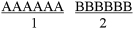
The first steps are to list the events in sequential order and count the number of runs. A run is a sequence of the same event written one or more times. For example, compare two event sequences. The first sequence is written AAAAAABBBBBB.
Then, separate the sequence into same groups as shown in Figure 9.1. There are two runs in this example, R = 2. This is a trend pattern in which events are clustered and it does not represent random behavior.
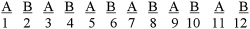
Consider a second event sequence written ABABABABABAB. Again, separate the events into same groups (see Fig. 9.2) to determine the number of runs. There are 12 runs in this example, R = 12. This is a cyclical pattern and does not represent random behavior either. As illustrated in the two examples earlier, too few or too many runs lack randomness.
A run can also describe how a sequence of events occurs in relation to a custom value. Use two symbols, such as A and B, to define whether an event exceeds or falls below the custom value. A simple example may reference the freezing point of water where A = temperatures above 0°C and B = temperatures below 0°C. In this example, simply list the events in order and determine the number of runs as described earlier.
After the number of runs is determined, it must be examined for significance. We may use a table of critical values (see Table B.10 in Appendix B). However, if the numbers of values in each sample, n1 or n2, exceed those available from the table, then a large sample approximation may be performed. For large samples, compute a z-score and use a table with the normal distribution (see Table B.1 in Appendix B) to obtain a critical region of z-scores. Formula 9.1, Fomula 9.2, Formula 9.3, Formula 9.4, and Formula 9.5 are used to find the z-score of a runs test for large samples:
where ![]() is the mean value of runs, n1 is the number of times the first event occurred, and n2 is the number of times the second event occurred;
is the mean value of runs, n1 is the number of times the first event occurred, and n2 is the number of times the second event occurred;
where sR is the standard deviation of runs;
where z* is the z-score for a normal approximation of the data, R is the number of runs, and h is the correction for continuity, ±0.5,
where
and
9.3.1 Sample Runs Test (Small Data Samples)
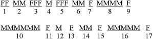
The following study seeks to examine gender bias in science instruction. A male science teacher was observed during a typical class discussion. The observer noted the gender of the student that the teacher called on to answer a question. In the course of 15 min, the teacher called on 10 males and 10 females. The observer noticed that the science teacher called on equal numbers of males and females, but he wanted to examine the data for a pattern. To determine if the teacher used a random order to call on students with regard to gender, he used a runs test for randomness. Using M for male and F for female, the sequence of student recognition by the teacher is MFFMFMFMFFMFFFMMFMMM.
9.3.1.1 State the Null and Research Hypotheses
The null hypothesis states that the sequence of events is random. The research hypothesis states that the sequence of events is not random.
The null hypothesis is
HO: The sequence in which the teacher calls on males and females is random.
The research hypothesis is
HA: The sequence in which the teacher calls on males and females is not random.
9.3.1.2 Set the Level of Risk (or the Level of Significance) Associated with the Null Hypothesis
The level of risk, also called an alpha (α), is frequently set at 0.05. We will use α = 0.05 in our example. In other words, there is a 95% chance that any observed statistical difference will be real and not due to chance.
9.3.1.3 Choose the Appropriate Test Statistic
The observer is examining the data for randomness. Therefore, he is using a runs test for randomness.
9.3.1.4 Compute the Test Statistic
First, determine the number of runs, R. It is helpful to separate the events as shown in Figure 9.3. The number of runs in the sequence is R = 13.

9.3.1.5 Determine the Value Needed for Rejection of the Null Hypothesis Using the Appropriate Table of Critical Values for the Particular Statistic
Since the sample sizes are small, we refer to Table B.10 in Appendix B, which lists the critical values for the runs test. There were 10 males (n1) and 10 females (n2). The critical values are found on the table at the point for n1 = 10 and n2 = 10. We set α = 0.05. The critical region for the runs test is 6 < R < 16. If the number of runs, R, is 6 or less, or 16 or greater, we reject our null hypothesis.
9.3.1.6 Compare the Obtained Value with the Critical Value
We found that R = 13. This value is within our critical region (6 < R < 16). Therefore, we do not reject the null hypothesis.
9.3.1.7 Interpret the Results
We did not reject the null hypothesis, suggesting that the sequence of events is random. Therefore, we can state that the order in which the science teacher calls on males and females is random.
9.3.1.8 Reporting the Results
The reporting of results for the runs test should include such information as the sample sizes for each group, the number of runs, and the p-value with respect to α.
For this example, the runs test indicated that the sequence was random (R = 13, n1 = 10, n2 = 10, p > 0.05). Therefore, the study provides evidence that the science teacher was demonstrating no gender bias.
9.3.2 Performing the Runs Test Using SPSS
We will analyze the data from the example earlier using SPSS.
9.3.2.1 Define Your Variables
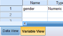
First, click the “Variable View” tab at the bottom of your screen. Then, type the names of your variables in the “Name” column. As seen in Figure 9.4, we call our variable “gender.”
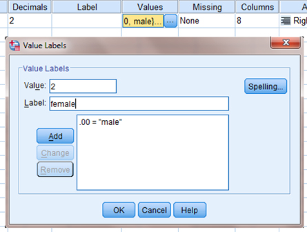
Next, we establish a grouping variable to differentiate between males and females. When establishing a grouping variable, it is often easiest to assign each group a whole number value. As shown in Figure 9.5, our groups are “male” and “female.” First, we select the “Values” column and click the gray square. Then, we set a value of 0 to represent “male” and a value of 2 to represent “female.” We use the “Add” button to move each of the value labels to the list. We did not choose the value of 1 since we will use it in step 3 as a reference (custom value) to compare the events. Once we finish, we click the “OK” button to return to the SPSS Variable View.
9.3.2.2 Type in Your Values
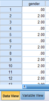
Click the “Data View” tab at the bottom of your screen (see Figure 9.6). Type the values into the column in the same order they occurred. Remember that we type 0 for “male” and 2 for “female.”
9.3.2.3 Analyze Your Data
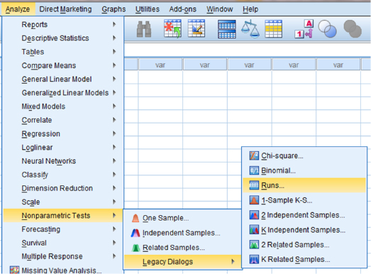
As shown in Figure 9.7, use the pull-down menus to choose “Analyze,” “Nonparametric Tests,” “Legacy Dialogs,” and “Runs….”
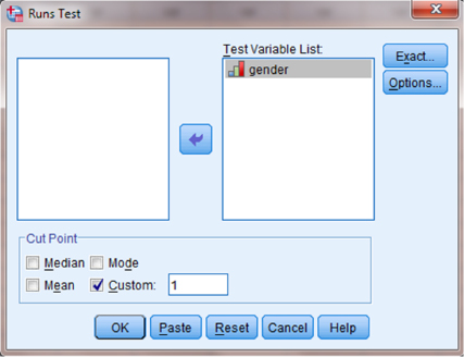
The runs test required a reference point to compare the events. As shown in Figure 9.8 under “Cut Point,” uncheck “Median” and check the box next to “Custom:.” Type a value in the box that is between the events' assigned values. For our example, we used 0 and 2 for the events' values, so type a custom value of 1. Next, select the variable and use the arrow button to place it with your data values in the box labeled “Test Variable List.” In our example, we choose the variable “gender.” Finally, click “OK” to perform the analysis.
9.3.2.4 Interpret the Results from the SPSS Output Window
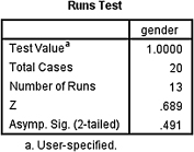
The runs test output table (see SPSS Output 9.1) returns the total number of observations (N = 20) and the number of runs (R = 13). SPSS also calculates the z-score (z* = 0.689) and the two-tailed significance (p = 0.491).
9.3.2.5 Determine the Observation Frequencies for Each Event
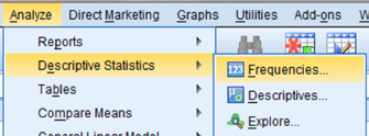
In order to determine the number of observations for each event, an additional set of steps is required. As shown in Figure 9.9, use the pull-down menus to choose “Analyze,” “Descriptive Statistics,” and “Frequencies….”
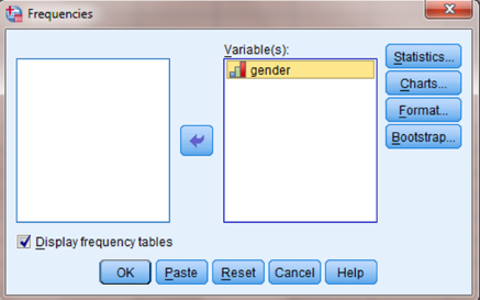
Next, use the arrow button to place the variable with your data values in the box labeled “Variable(s):” as shown in Figure 9.10. Like before, we choose the variable “gender.” Finally, click “OK” to perform the analysis.
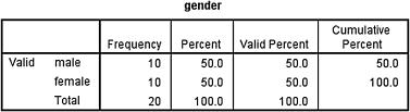
The second output table (see SPSS Output 9.2) displays the frequencies for each event. Based on the results from SPSS, the runs test indicated that the sequence was random (R = 13, n1 = 10, n2 = 10, p > 0.05). Therefore, the science teacher randomly chose between males and females when calling on students.
9.3.3 Sample Runs Test (Large Data Samples)
The previous study investigating gender bias was replicated. This time, however, a different male teacher was observed and the observation occurred over a longer period of time. As before, the observer noted the gender of the student that the teacher called on to answer a question. In the course of 30 min, the teacher called on 23 males and 14 females. We will once again examine the data for a pattern and use a runs test to examine student recognition with respect to gender. This time, however, we will use a large sample approximation since at least one sample size is large. Using M for male and F for female, the sequence of student recognition by the teacher is FFMMFFFMFFFMMFMMMMFMMMMMMFMFMMFMMMMMF.
9.3.3.1 State the Null and Research Hypotheses
The null hypothesis states that the sequence of events is random. The research hypothesis states that the sequence of events is not random.
The null hypothesis is
HO: The sequence in which the teacher calls on males and females is random.
The research hypothesis is
HA: The sequence in which the teacher calls on males and females is not random.
9.3.3.2 Set the Level of Risk (or the Level of Significance) Associated with the Null Hypothesis
The level of risk, also called an alpha (α), is frequently set at 0.05. We will use α = 0.05 in our example. In other words, there is a 95% chance that any observed statistical difference will be real and not due to chance.
9.3.3.3 Choose the Appropriate Test Statistic
The observer is examining the data for randomness. Therefore, he is using a runs test for randomness.
9.3.3.4 Compute the Test Statistic
First, determine the number of runs, R. It is helpful to separate the events as shown in Figure 9.11. The number of runs in the sequence is R = 17.
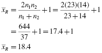
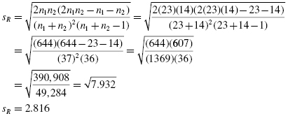
Our number of values exceeds those available from our critical value table for the runs test (Table B.10 in Appendix B is limited to n1 ≤ 20 and n2 ≤ 20). Therefore, we will find a z-score for our data using a normal approximation. First, we must find the mean ![]() and the standard deviation sR for the data:
and the standard deviation sR for the data:
and
Next, we calculate a z-score. We use the correction for continuity, mean, standard deviation, and number of runs (R = 17) to calculate a z-score. The only value that we still need is the correction for continuity h. Recall that h = +0.5 if R < (2n1n2/(n1 + n2) + 1), and h = −0.5 if R > (2n1n2/(n1 + n2) + 1). In our example, 2n1n2/(n1 + n2) + 1 = 2(23)(14)/(23 + 14) + 1 = 18.4. Since 17 < 18.4, we choose h = +0.5.
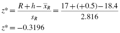
Now, we use our z-score formula with correction for continuity:
9.3.3.5 Determine the Value Needed for Rejection of the Null Hypothesis Using the Appropriate Table of Critical Values for the Particular Statistic
Table B.1 in Appendix B is used to establish the critical region of z-scores. For a two-tailed test with α = 0.05, we must not reject the null hypothesis if −1.96 ≤ z* ≤ 1.96.
9.3.3.6 Compare the Obtained Value with the Critical Value
We find that z* is within the critical region of the distribution, −1.96 ≤ −0.3196 ≤ 1.96. Therefore, we do not reject the null hypothesis. This suggests that the order in which the science teacher calls on males and females is random.
9.3.3.7 Interpret the Results
We did not reject the null hypothesis, suggesting that the sequence of events is random. Therefore, our data indicate that the order in which the science teacher calls on males and females is random.
9.3.3.8 Reporting the Results
Based on our analysis, the runs test indicated that the sequence was random (R = 17, n1 = 23, n2 = 14, p > 0.05). Therefore, the study provides evidence that the science teacher was demonstrating no gender bias.
9.3.4 Sample Runs Test Referencing a Custom Value
The science teacher in the earlier example wishes to examine the pattern of an “at-risk” student's weekly quiz performance. A passing quiz score is 70. Sometimes the student failed and other times he passed. The teacher wished to determine if the student's performance is random or not. Table 9.1 shows the student's weekly quiz scores for a 12-week period.
| Week | Student quiz scores |
|---|---|
| 1 | 65 |
| 2 | 55 |
| 3 | 95 |
| 4 | 15 |
| 5 | 75 |
| 6 | 65 |
| 7 | 80 |
| 8 | 75 |
| 9 | 60 |
| 10 | 55 |
| 11 | 75 |
| 12 | 80 |
9.3.4.1 State the Null and Research Hypotheses
The null hypothesis states that the sequence of events is random. The research hypothesis states that the sequence of events is not random.
The null hypothesis is
HO: The sequence in which the student passes and fails a weekly science quiz is random.
The research hypothesis is
HA: The sequence in which the student passes and fails a weekly science quiz is not random.
9.3.4.2 Set the Level of Risk (or the Level of Significance) Associated with the Null Hypothesis
The level of risk, also called an alpha (α), is frequently set at 0.05. We will use α = 0.05 in our example. In other words, there is a 95% chance that any observed statistical difference will be real and not due to chance.
9.3.4.3 Choose the Appropriate Test Statistic
The observer is examining the data for randomness. Therefore, he is using a runs test for randomness.
9.3.4.4 Compute the Test Statistic
The custom value is 69.9 since a passing quiz score is 70. We must identify which quiz scores fall above the custom score and which quiz scores fall below it. As shown in Table 9.2, we mark the quiz scores that fall above the custom score with + and the quiz scores that fall below with −.
| Week | Student quiz scores | Relation to custom score |
|---|---|---|
| 1 | 65 | − |
| 2 | 55 | − |
| 3 | 95 | + |
| 4 | 15 | − |
| 5 | 75 | + |
| 6 | 65 | − |
| 7 | 80 | + |
| 8 | 75 | + |
| 9 | 60 | − |
| 10 | 55 | − |
| 11 | 70 | + |
| 12 | 80 | + |
Then, we count the number of runs, R. The number of runs in the sequence earlier is R = 8.
9.3.4.5 Determine the Value Needed for Rejection of the Null Hypothesis Using the Appropriate Table of Critical Values for the Particular Statistic
Since the sample sizes are small, we refer to Table B.10 in Appendix B, which lists the critical values for the runs test. The critical values are found on the table at the point for n1 = 6 and n2 = 6. We set α = 0.05. The critical region for the runs test is 3 < R < 11. If the number of runs, R, is 3 or less, or 11 or greater, we reject our null hypothesis.
9.3.4.6 Compare the Obtained Value with the Critical Value
We found that R = 8. This value is within our critical region (3 < R < 11). Therefore, we must not reject the null hypothesis.
9.3.4.7 Interpret the Results
We did not reject the null hypothesis, suggesting that the sequence of events is random. Therefore, we can state that based on a passing score of 70, the student's weekly science quiz performance is random.
9.3.4.8 Reporting the Results
For this example, the runs test indicated that the sequence was random (R = 8, n1 = 6, n2 = 6, p > 0.05). Therefore, the evidence suggests that the pattern of the student's weekly science quiz performance is random in terms of achieving a passing score of 70.
9.3.5 Performing the Runs Test for a Custom Value Using SPSS
We will analyze the data from the earlier example using SPSS.
9.3.5.1 Define Your Variables
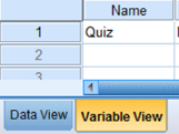
First, click the “Variable View” tab at the bottom of your screen. As shown in Figure 9.12, type the names of your variables in the “Name” column. We call our variable “Quiz.”
9.3.5.2 Type in Your Values
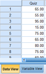
Click the “Data View” tab at the bottom of your screen, as shown in Figure 9.13. Type the values into the column in the same order they occurred.
9.3.5.3 Analyze Your Data
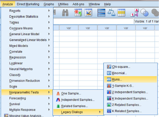
As shown in Figure 9.14, use the pull-down menus to choose “Analyze,” “Nonparametric Tests,” “Legacy Dialogs,” and “Runs….”
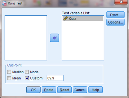
As shown in Figure 9.15 under “Cut Point,” uncheck “Median” and check the box next to “Custom:.” Type the custom value in the box. For our example, we use a custom value of 69.9. Next, use the arrow button to place the variable with your data values in the box labeled “Test Variable List.” In our example, we choose the variable “Quiz.” Finally, click the “OK” button to perform the analysis.
9.3.5.4 Interpret the Results from the SPSS Output Window
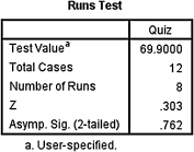
The runs test output table (see SPSS Output 9.3) returns the custom test value (69.9), the total number of observations (N = 12), and the number of runs (R = 8). SPSS also calculates the z-score (z* = 0.303) and the two-tailed significance (p = 0.762).
9.3.5.5 Determine the Observation Frequencies for Each Event
In order to determine the number of observations for each event, an additional set of steps is required.
As shown in Figure 9.16, use the pull-down menus to choose “Analyze,” “Descriptive Statistics,” and “Frequencies….”
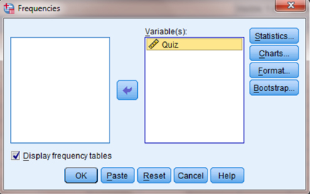
Next, use the arrow button to place the variable with your data values in the box labeled “Variable(s):,” as shown in Figure 9.17. The variable test is called “Quiz.” Finally, click “OK” to perform the analysis.
The second output table (see SPSS Output 9.4) displays the frequencies for each value. You must count the number of values above the custom value and the number values below it to determine the frequency for each event.
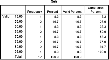
Based on the results from SPSS, the runs test indicated that the sequence was random (R = 8, n1 = 6, n2 = 6, p > 0.05). Therefore, the pattern of the student's weekly science quiz performance is random in terms of achieving a passing score of 70.
9.4 Examples from the Literature
Listed are varied examples of the nonparametric procedures described in this chapter. We have summarized each study's research problem and researchers' rationale(s) for choosing a nonparametric approach. We encourage you to obtain these studies if you are interested in their results.
Dorsey-Palmateer and Smith (2004) called into question a classical statistics experiment that debunked a commonly held belief that basketball players' shooting accuracy is based on the performance immediately preceding a given shot. The authors explored this notion of hot hands among professional bowlers. They examined a series of rolls and differentiate between strikes and nonstrikes. They used a runs test to analyze the sequence of bowlers' performance for randomness.
Vergin (2000) explored the presence of momentum among Major League Baseball (MLB) teams and National Basketball Association (NBA) teams. He described momentum as the tendency for a winning team to continue to win and a losing team to continue to lose. Therefore, he used a Wald–Wolfowitz runs test to examine the winning and losing streaks of the 28 MLB teams in 1996 and of the 29 NBA teams during the 1996–1997 and 1997–1998 seasons.
Pollay et al. (1992) investigated the possibility that cigarette companies segregated and segmented advertising efforts toward black consumers. They used a runs test to compare the change in annual frequency of cigarette ads that appeared in Life Magazine versus Ebony.
9.5 Summary
The runs test is a statistical procedure for examining a series of events for randomness. This nonparametric test has no parametric equivalent. In this chapter, we described how to perform and interpret a runs test for both small samples and large samples. We also explained how to perform the procedure using SPSS. Finally, we offered varied examples of these nonparametric statistics from the literature.
9.6 Practice Questions
1. Represented in the data is the daily performance of a popular stock. Letter A represents a gain and letter B represents a loss. Use a runs test to analyze the stock's performance for randomness. Set α = 0.05. Report the results.
BAABBAABBBBBAABAAAAB
2. A machine on an automated assembly line produces a unique type of bolt. If the machine fails more than three times in an hour, the total production on the line is slowed down. The machine has often exceeded the number of acceptable failures for the last week. The machine is expensive and more cost-effective to repair, but the maintenance crew cannot find the problem. The plant manager asks you to determine if the failure rates are random or if a pattern exists. Table 9.3 shows the number of failures per hour for a 24-h period.
Use a runs test with a custom value of 3.1 to analyze the acceptable/unacceptable failure rate for randomness. Set α = 0.05. Report the results.
| Hour | Number of failures |
|---|---|
| 1 | 6 |
| 2 | 4 |
| 3 | 2 |
| 4 | 2 |
| 5 | 7 |
| 6 | 5 |
| 7 | 7 |
| 8 | 9 |
| 9 | 2 |
| 10 | 0 |
| 11 | 0 |
| 12 | 0 |
| 13 | 7 |
| 14 | 6 |
| 15 | 5 |
| 16 | 9 |
| 17 | 1 |
| 18 | 0 |
| 19 | 1 |
| 20 | 8 |
| 21 | 5 |
| 22 | 9 |
| 23 | 4 |
| 24 | 5 |
9.7 Solutions to Practice Questions
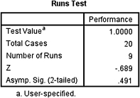
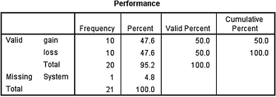
1. The results from the analysis are displayed in SPSS Output 9.5a and SPSS Output 9.5b.
The sequence of the stock's gains and losses was random (R = 9, n1 = 10, n2 = 10, p > 0.05).
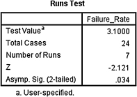
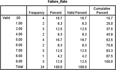
2. The results from the analysis are displayed in SPSS Output 9.6a and SPSS Output 9.6b.
The sequence of the machine's acceptable/unacceptable failure rate was not random (R = 7, n1 = 9, n2 = 15, p < 0.05).