CHAPTER 3
Comparing Two Related Samples: The Wilcoxon Signed Rank and the Sign Test
3.1 Objectives
In this chapter, you will learn the following items:
- How to compute the Wilcoxon signed rank test.
- How to perform the Wilcoxon signed rank test using SPSS®.
- How to construct a median confidence interval based on the Wilcoxon signed rank test for matched pairs.
- How to compute the sign test.
- How to perform the sign test using SPSS.
3.2 Introduction
Imagine that you give an attitude test to a small group of people. After you deliver some type of treatment, say, a daily vitamin C supplement for several weeks, you give that same group of people another attitude test. Finally, you compare the two measures of attitude to see if there is any type of difference between the two sets of scores.
The two sets of test scores in the previous scenario are related or paired. This is because each person was tested twice. In other words, each test score in one group of scores has another test score counterpart. The Wilcoxon signed rank test and the sign test are nonparametric statistical procedures for comparing two samples that are paired or related. The parametric equivalent to these tests goes by names such as the Student's t-test, t-test for matched pairs, t-test for paired samples, or t-test for dependent samples.
In this chapter, we will describe how to perform and interpret a Wilcoxon signed rank test and a sign test, using both small samples and large samples. In addition, we demonstrate the procedures for performing both tests using SPSS. Finally, we offer varied examples of these nonparametric statistics from the literature.
3.3 Computing the Wilcoxon Signed Rank Test Statistic
The formula for computing the Wilcoxon T for small samples is shown in Formula 3.1. The signed ranks are the values that are used to compute the positive and negative values in the formula:
where ΣR+ is the sum of the ranks with positive differences and ΣR− is the sum of the ranks with negative differences.
After the T statistic is computed, it must be examined for significance. We may use a table of critical values (see Table B.3 in Appendix B). However, if the numbers of pairs n exceeds those available from the table, then a large sample approximation may be performed. For large samples, compute a z-score and use a table with the normal distribution (see Table B.1 in Appendix B) to obtain a critical region of z-scores. Formula 3.2, Formula 3.3, and Formula 3.4 are used to find the z-score of a Wilcoxon signed rank test for large samples:
where ![]() is the mean and n is the number of matched pairs included in the analysis,
is the mean and n is the number of matched pairs included in the analysis,
where sT is the standard deviation,
where z* is the z-score for an approximation of the data to the normal distribution and T is the T statistic.
At this point, the analysis is limited to identifying the presence or absence of a significant difference between the groups and does not describe the strength of the treatment. We can consider the effect size (ES) to determine the degree of association between the groups. We use Formula 3.5 to calculate the ES:
where |z| is the absolute value of the z-score and n is the number of matched pairs included in the analysis.
The ES ranges from 0 to 1. Cohen (1988) defined the conventions for ES as small = 0.10, medium = 0.30, and large = 0.50. (Correlation coefficient and ES are both measures of association. See Chapter 7 concerning correlation for more information on Cohen's assignment of ES's relative strength.)
3.3.1 Sample Wilcoxon Signed Rank Test (Small Data Samples)
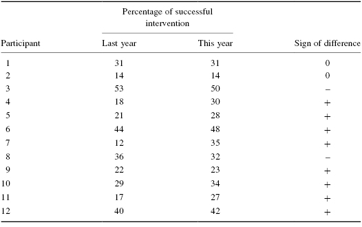
The counseling staff of Clear Creek County School District has implemented a new program this year to reduce bullying in their elementary schools. The school district does not know if the new program resulted in improvement or deterioration. In order to evaluate the program's effectiveness, the school district has decided to compare the percentage of successful interventions last year before the program began with the percentage of successful interventions this year with the program in place. In Table 3.1, the 12 elementary school counselors, or participants, reported the percentage of successful interventions last year and the percentage this year.
| Participants | Percentage of successful interventions | |
|---|---|---|
| Last year | This year | |
| 1 | 31 | 31 |
| 2 | 14 | 14 |
| 3 | 53 | 50 |
| 4 | 18 | 30 |
| 5 | 21 | 28 |
| 6 | 44 | 48 |
| 7 | 12 | 35 |
| 8 | 36 | 32 |
| 9 | 22 | 23 |
| 10 | 29 | 34 |
| 11 | 17 | 27 |
| 12 | 40 | 42 |
The samples are relatively small, so we need a nonparametric procedure. Since we are comparing two related, or paired, samples, we will use the Wilcoxon signed rank test.
3.3.1.1 State the Null and Research Hypotheses
The null hypothesis states that the counselors reported no difference in the percentages last year and this year. The research hypothesis states that the counselors observed some differences between this year and last year. Our research hypothesis is a two-tailed, nondirectional hypothesis because it indicates a difference, but in no particular direction.
The null hypothesis is
HO: μD = 0
The research hypothesis is
HA: μD ≠ 0
3.3.1.2 Set the Level of Risk (or the Level of Significance) Associated with the Null Hypothesis
The level of risk, also called an alpha (α), is frequently set at 0.05. We will use α = 0.05 in our example. In other words, there is a 95% chance that any observed statistical difference will be real and not due to chance.
3.3.1.3 Choose the Appropriate Test Statistic
The data are obtained from 12 counselors, or participants, who are using a new program designed to reduce bullying among students in the elementary schools. The participants reported the percentage of successful interventions last year and the percentage this year. We are comparing last year's percentages with this year's percentages. Therefore, the data samples are related or paired. In addition, sample sizes are relatively small. Since we are comparing two related samples, we will use the Wilcoxon signed rank test.
3.3.1.4 Compute the Test Statistic
First, compute the difference between each sample pair. Then, rank the absolute value of those computed differences. Using this method, the differences of zero are ignored when ranking. We have done this in Table 3.2.
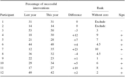
Compute the sum of ranks with positive differences. Using Table 3.2, the ranks with positive differences are 9, 7, 4.5, 10, 1, 6, 8, and 2. When we add all of the ranks with positive difference we get ΣR+ = 47.5.
Compute the sum of ranks with negative differences. The ranks with negative differences are 3 and 4.5. The sum of ranks with negative difference is ΣR− = 7.5.
The obtained value is the smaller of the two rank sums. Therefore, the Wilcoxon is T = 7.5.
3.3.1.5 Determine the Value Needed for Rejection of the Null Hypothesis Using the Appropriate Table of Critical Values for the Particular Statistic
Since the sample sizes are small, we use Table B.3 in Appendix B, which lists the critical values for the Wilcoxon T. As noted earlier in Table 3.2, the two counselors with score differences of zero were discarded. This reduces our sample size to n = 10. In this case, we look for the critical value under the two-tailed test for n = 10 and α = 0.05. Table B.3 returns a critical value for the Wilcoxon test of T = 8. An obtained value that is less than or equal to 8 will lead us to reject our null hypothesis.
3.3.1.6 Compare the Obtained Value with the Critical Value
The critical value for rejecting the null hypothesis is 8 and the obtained value is T = 7.5. If the critical value equals or exceeds the obtained value, we must reject the null hypothesis. If instead, the critical value is less than the obtained value, we must not reject the null hypothesis. Since the critical value exceeds the obtained value, we must reject the null hypothesis.
3.3.1.7 Interpret the Results
We rejected the null hypothesis, suggesting that a real difference exists between last year's percentages and this year's percentages. In addition, since the sum of the positive difference ranks (ΣR+) was larger than the negative difference ranks (ΣR−), the difference is positive, showing a positive impact of the program. Therefore, our analysis provides evidence that the new bullying program is providing positive benefits toward the improvement of student behavior as perceived by the school counselors.
3.3.1.8 Reporting the Results
When reporting the findings, include the T statistic, sample size, and p-value's relation to α. The directionality of the difference should be expressed using the sum of the positive difference ranks (ΣR+) and sum of the negative difference ranks (ΣR−).
For this example, the Wilcoxon signed rank test (T = 7.5, n = 12, p < 0.05) indicated that the percentage of successful interventions was significantly different. In addition, the sum of the positive difference ranks (ΣR+ = 47.5) was larger than the sum of the negative difference ranks (ΣR− = 7.5), showing a positive impact from the program. Therefore, our analysis provides evidence that the new bullying program is providing positive benefits toward the improvement of student behavior as perceived by the school counselors.
3.3.2 Confidence Interval for the Wilcoxon Signed Rank Test
The American Psychological Association (2001) has suggested that researchers report the confidence interval for research data. A confidence interval is an inference to a population in terms of an estimation of sampling error. More specifically, it provides a range of values that fall within the population with a level of confidence of 100(1 − α)%.
A median confidence interval can be constructed based on the Wilcoxon signed rank test for matched pairs. In order to create this confidence interval, all of the possible matched pairs (Xi,Xj) are used to compute the differences Di = Xi − Xj. Then, compute all of the averages uij of two difference scores using Formula 3.6. There will be a total of [n(n − 1)/2] + n averages.
We will perform a 95% confidence interval using the sample Wilcoxon signed rank test with a small data sample (as stated earlier). Table 3.1 provides the values for obtaining our confidence interval. We begin by using Formula 3.6 to compute all of the averages uij of two difference scores. For example,
Table 3.3 shows each value of uij.
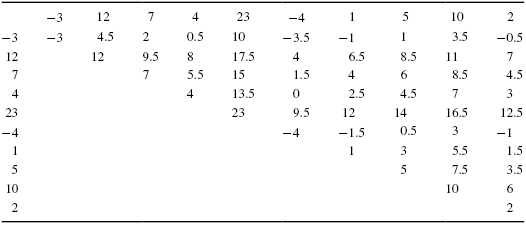
Next, arrange all of the averages in order from smallest to largest. We have arranged all of the values for uij in Table 3.4.
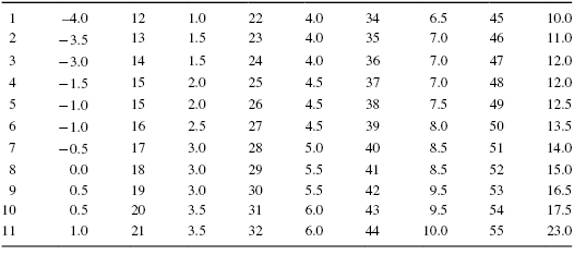
The median of the ordered averages gives a point estimate of the population median difference. The median of this distribution is 4.5, which is the point estimate of the population.
Use Table B.3 in Appendix B to find the endpoints of the confidence interval. First, determine T from the table that corresponds with the sample size and desired confidence such that p = α/2. We seek to find a 95% confidence interval. For our example, n = 10 and p = 0.05/2. The table provides T = 8.
The endpoints of the confidence interval are the Kth smallest and the Kth largest values of uij, where K = T + 1. For our example, K = 8 + 1 = 9. The ninth value from the bottom is 0.5 and the ninth value from the top is 12.0. Based on these findings, it is estimated with 95% confident that the difference of successful interventions due to the new bullying programs lies between 0.5 and 12.0.
3.3.3 Sample Wilcoxon Signed Rank Test (Large Data Samples)
Hearing of Clear Creek School District's success with their antibullying program, Jonestown School District has implemented the program this year to reduce bullying in their own elementary schools. The Jonestown School District evaluates their program's effectiveness by comparing the percentage of successful interventions last year before the program began with the percentage of successful interventions this year with the program in place. In Table 3.5, the 25 elementary school counselors, or participants, reported the percentage of successful interventions last year and the percentage this year.
| Participant | Percentage of successful interventions | |
|---|---|---|
| Last year | This year | |
| 1 | 53 | 50 |
| 2 | 18 | 43 |
| 3 | 21 | 28 |
| 4 | 44 | 48 |
| 5 | 12 | 35 |
| 6 | 36 | 32 |
| 7 | 22 | 23 |
| 8 | 29 | 34 |
| 9 | 17 | 27 |
| 10 | 10 | 42 |
| 11 | 38 | 44 |
| 12 | 37 | 16 |
| 13 | 19 | 33 |
| 14 | 37 | 50 |
| 15 | 28 | 20 |
| 16 | 15 | 27 |
| 17 | 25 | 27 |
| 18 | 38 | 30 |
| 19 | 40 | 51 |
| 20 | 30 | 50 |
| 21 | 23 | 45 |
| 22 | 41 | 20 |
| 23 | 31 | 49 |
| 24 | 28 | 43 |
| 25 | 14 | 30 |
We will use the same nonparametric procedure to analyze the data. However, use a large sample (n ≥ 20) approximation.
3.3.3.1 State the Null and Research Hypotheses
The null hypothesis states that the counselors reported no difference in the percentages last year and this year. The research hypothesis states that the counselors observed some differences between this year and last year. Our research hypothesis is a two-tailed, nondirectional hypothesis because it indicates a difference, but in no particular direction.
The null hypothesis is
HO: μD = 0
The research hypothesis is
HA: μD ≠ 0
3.3.3.2 Set the Level of Risk (or the Level of Significance) Associated with the Null Hypothesis
The level of risk, also called an alpha (α), is frequently set at 0.05. We will use α = 0.05 in our example. In other words, there is a 95% chance that any observed statistical difference will be real and not due to chance.
3.3.3.3 Choose the Appropriate Test Statistic
The data are obtained from 25 counselors, or participants, who are using a new program designed to reduce bullying among students in the elementary schools. The participants reported the percentage of successful interventions last year and the percentage this year. We are comparing last year's percentages with this year's percentages. Therefore, the data samples are related or paired. Since we are comparing two related samples, we will use the Wilcoxon signed rank test.
3.3.3.4 Compute the Test Statistic
First, compute the difference between each sample pair. Then, rank the absolute value of those computed differences. We have done this in Table 3.6.
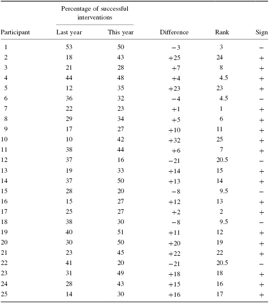
Compute the sum of ranks with positive differences. Using Table 3.6, when we add all of the ranks with positive difference, we get ΣR+ = 257.5.
Compute the sum of ranks with negative differences. The ranks with negative differences are 3, 4.5, 9.5, 9.5, 20.5, and 20.5. The sum of ranks with negative difference is ΣR− = 67.5.
The obtained value is the smaller of these two rank sums. Thus, the Wilcoxon T = 67.5.
Since our sample size is larger than 20, we will approximate it to a normal distribution. Therefore, we will find a z-score for our data using a normal approximation. We must find the mean ![]() and the standard deviation sT for the data:
and the standard deviation sT for the data:
and
Next, we use the mean, standard deviation, and the T-test statistic to calculate a z-score. Remember, we are testing the hypothesis that there is no difference in ranks of percentages of successful interventions between last year and this year:
3.3.3.5 Determine the Value Needed for Rejection of the Null Hypothesis Using the Appropriate Table of Critical Values for the Particular Statistic
Table B.1 in Appendix B is used to establish the critical region of z-scores. For a two-tailed test with α = 0.05, we must not reject the null hypothesis if −1.96 ≤ z* ≤ 1.96.
3.3.3.6 Compare the Obtained Value to the Critical Value
We find that z* is not within the critical region of the distribution, −2.56 < −1.96. Therefore, we reject the null hypothesis. This suggests a difference in the percentage of successful interventions after the program was implemented.
3.3.3.7 Interpret the Results
We rejected the null hypothesis, suggesting that a real difference exists between last year's percentages and this year's percentages. In addition, since the sum of the positive difference ranks (ΣR+) was larger than the negative difference ranks (ΣR−), the difference is positive, showing a positive impact of the program. Therefore, our analysis provides evidence that the new bullying program is providing positive benefits toward the improvement of student behavior as perceived by the school counselors.
At this point, the analysis is limited to identifying the presence or absence of a significant difference between the groups. In other words, the statistical test's level of significance does not describe the strength of the treatment. The American Psychological Association (2001), however, has called for a measure of the strength called the ES.
We can consider the ES for this large sample test to determine the degree of association between the groups. We use Formula 3.5 to calculate the ES. For the example, |z| = 2.56 and n = 25:
Our ES for the matched-pair samples is 0.51. This value indicates a high level of association between the percentage of successful interventions before and after the implementation of the new bullying program.
3.3.3.8 Reporting the Results
For this example, the Wilcoxon signed rank test (T = 67.5, n = 25, p < 0.05) indicated that the percentage of successful interventions was significantly different. In addition, the sum of the positive difference ranks (ΣR+ = 257.5) was larger than the sum of the negative difference ranks (ΣR− = 67.5), showing a positive impact from the program. Moreover, the ES for the matched-pair samples was 0.51. Therefore, our analysis provides evidence that the new bullying program is providing positive benefits toward the improvement of student behavior as perceived by the school counselors.
3.4 Computing the Sign Test
You can analyze related samples more efficiently by reducing values to dichotomous results (“yes” or “no”) or (“+” or “−”). The sign test allows you to perform that analysis. Our procedure for performing the sign test is based on the method described by Gibbons and Chakraborti (2010).
We begin the procedure for performing a sign test by identifying whether each set from the related data samples demonstrates a positive difference, a negative difference, or no difference at all. Then, we find the sum of the positive differences np and the sum of negative differences nn. Cases with no difference are ignored.
We perform the next part of the analysis based on the sum of differences. If np + nn = 0, then the one-sided probability is p = 0.5. If 0 < np + nn < 25, then p is calculated recursively from the binomial probability function using Formula 3.7. Table B.9 in Appendix B includes several factorials to simplify computation:
where n = np + nn and p is the probability of event occurrence.
If np + nn ≥ 25, we use Formula 3.8:
Formula 3.8 approximates a binomial distribution to the normal distribution. However, the binomial distribution is a discrete distribution, while the normal distribution is continuous. More to the point, discrete values deal with heights but not widths, while the continuous distribution deals with both heights and widths. The correction adds or subtracts 0.5 of a unit from each discrete X-value to fill the gaps and make it continuous.
The one sided p-value is p1 = 1 − Φ|zc|, where Φ|zc| is the area under the respective tail of the normal distribution at zc. The two-sided p-value is p = 2p1.
3.4.1 Sample Sign Test (Small Data Samples)
To present the process for performing the sign test, we are going to use the data from Section 3.3.1, which used the Wilcoxon signed rank test. Recall that the sample involves 12 members of the counseling staff from Clear Creek County School District who are working on a program to improve response to bullying in the schools. The data from Table 3.1 are being reduced to a binomial distribution for use with the sign test. The relatively small sample size warrants a nonparametric procedure.
3.4.1.1 State the Null and Research Hypotheses
The null hypothesis states that the counselors reported no difference between positive or negative interventions between last year and this year. In other words, the changes in responses produce a balanced number of positive and negative differences. The research hypothesis states that the counselors observed some differences between this year and last year. Our research hypothesis is a two-tailed, nondirectional hypothesis because it indicates a difference, but in no particular direction.
The null hypothesis is
HO: p = 0.5
The research hypothesis is
HA: p ≠ 0.5
3.4.1.2 Set the Level of Risk (or the Level of Significance) Associated with the Null Hypothesis
The level of risk, also called an alpha (α), is frequently set at 0.05. We will use α = 0.05 in our example. In other words, there is a 95% chance that any observed statistical difference will be real and not due to chance.
3.4.1.3 Choose the Appropriate Test Statistic
Recall from Section 3.3.1 that the data are obtained from 12 counselors, or participants, who are using a new program designed to reduce bullying among students in the elementary schools. The participants reported the percentage of successful interventions last year and the percentage this year. We are comparing last year's percentages with this year's percentages. Therefore, the data samples are related or paired. In addition, sample sizes are relatively small. Since we are comparing two related samples, we will use the sign test.
3.4.1.4 Compute the Test Statistic
First, decide if there is a difference in intervention score from year 1 to year 2. Determine if the difference is positive or negative and put the sign of the difference in the sign column. If we count the number of ties or “0” differences among the group, we find only two with no difference from last year to this year. Ties are discarded.
Now, we count the number of positive and negative differences between last year and this year. Count the number of “+” or positive differences. When we look at Table 3.7, we see that eight participants showed positive differences, np = 8. Count the number of “−” or negative differences. When we look at Table 3.7, we see only two negative differences, nn = 2.
Next, we find the X-score at and beyond where the area under our binomial probability function is α = 0.05. Since we are performing a two-tailed test, we use 0.025 for each tail. We will calculate the probabilities associated with the binomial distribution for p = 0.5 and n = 10. We will demonstrate one of the calculations, but list the results for each value. To simplify calculation, use the table of factorials in Appendix B, Table B.9:
Notice that the values form a symmetric distribution with the median at P(5), as shown in Figure 3.1. Using this distribution, we find the p-values for each tail. To do that, we sum the probabilities for each tail until we find a probability equal to or greater than α/2 = 0.025. First, calculate P for pluses:
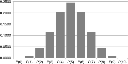
Second, calculate P for minuses:
Finally, calculate the obtained value p by combining the two tails:
3.4.1.5 Determine the Critical Value Needed for Rejection of the Null Hypothesis
In the example in this chapter, the two-tailed probability was computed and is compared with the level of risk specified earlier, α = 0.05.
3.4.1.6 Compare the Obtained Value with the Critical Value
The critical value for rejecting the null hypothesis is α = 0.05 and the obtained p-value is p = 0.1094. If the critical value is greater than the obtained value, we must reject the null hypothesis. If the critical value is less than the obtained value, we do not reject the null hypothesis. Since the critical value is less than the obtained value (p > α), we do not reject the null hypothesis.
3.4.1.7 Interpret the Results
We did not reject the null hypothesis, suggesting that no real difference exists between last year's and this year's percentages. There was no evidence of positive or negative intervention by counselors. These results differ from the data's analysis using the Wilcoxon signed rank test. A discussion about statistical power addresses those differences toward the end of this chapter.
3.4.1.8 Reporting the Results
When reporting the findings for the sign test, you should include the sample size, the number of pluses, minuses, and ties, and the probability of getting the obtained number of pluses and minuses.
For this example, the obtained value, p = 0.1094, was greater than the critical value, α = 0.05. Therefore, we did not reject the null hypothesis, suggesting that the new bullying program is not providing evidence of a change in student behavior as perceived by the school counselors.
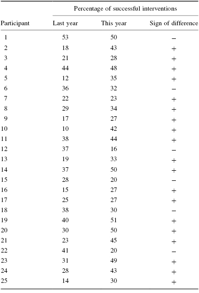
3.4.2 Sample Sign Test (Large Data Samples)
We are going to demonstrate a sign test with large samples using the data from the Wilcoxon signed rank test for large samples in Section 3.3.3. The data from the implementation of the bullying program in the Jonestown School District are presented in Table 3.8. The data are used to determine the effect of the bullying program from year 1 to year 2. If there is an increase in successful intervention, we will use a “+” to identify the positive difference in response. If there is a decrease in successful intervention in the response, we will identify a negative difference with a “−.” There are 25 participants in this study.
| Participant | Percentage of successful interventions | |
|---|---|---|
| Last year | This year | |
| 1 | 53 | 50 |
| 2 | 18 | 43 |
| 3 | 21 | 28 |
| 4 | 44 | 48 |
| 5 | 12 | 35 |
| 6 | 36 | 32 |
| 7 | 22 | 23 |
| 8 | 29 | 34 |
| 9 | 17 | 27 |
| 10 | 10 | 42 |
| 11 | 38 | 44 |
| 12 | 37 | 16 |
| 13 | 19 | 33 |
| 14 | 37 | 50 |
| 15 | 28 | 20 |
| 16 | 15 | 27 |
| 17 | 25 | 27 |
| 18 | 38 | 30 |
| 19 | 40 | 51 |
| 20 | 30 | 50 |
| 21 | 23 | 45 |
| 22 | 41 | 20 |
| 23 | 31 | 49 |
| 24 | 28 | 43 |
| 25 | 14 | 30 |
3.4.2.1 State the Null and Alternate Hypotheses
The null hypothesis states that there was no positive or negative effect of the bullying program on successful intervention. The research hypothesis states that either a positive or negative effect exists from the bullying program.
The null hypothesis is
HO: p = 0.5
The research hypothesis is
HA: p ≠ 0.5
3.4.2.2 Set the Level of Risk (or the Level of Significance) Associated with the Null Hypothesis
The level of risk, also called an alpha (α), is frequently set at 0.05. We will use α = 0.05 in our example. In other words, there is a 95% chance that any observed statistical difference will be real and not due to chance.
3.4.2.3 Choose the Appropriate Test Statistic
Recall from Section 3.3.3 that the data were obtained from 25 counselors, or participants, who were using a new program designed to reduce bullying among students in the elementary schools. The participants reported the percentage of successful interventions last year and the percentage this year. We are comparing last year's percentages with this year's percentages. Therefore, the data samples are related or paired. Since we are making dichotomous comparisons of two related samples, we will use the sign test.
3.4.2.4 Compute the Test Statistic
First, we determine the sign of the differences between last year and this year. Table 3.9 includes the column for the sign of the difference for each participant. Next, we count the numbers of positive and negative differences. We find six negative differences, nn = 6, and 19 positive differences, np = 19.
Since the sample size is n ≥ 25, we will use a z-score approximation of the binomial distribution. The binomial distribution becomes an approximation of the normal distribution as n becomes large and p is not too close to the 0 or 1 values. If this approximation is used, P(Y ≤ k) is obtained by computing the corrected z-score for the given data that are as extreme or more extreme than the data given:
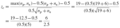
Next, we find the one-sided p-value. Table B.1 is used to establish Φ|zc|.
We now multiply two times the one-sided p-value to find the two-sided p-value:
3.4.2.5 Determine the Critical Value Needed for Rejection of the Null Hypothesis
In the example in this chapter, the two-tailed probability was computed and compared with the level of risk specified earlier, α = 0.05.
3.4.2.6 Compare the Obtained Value with the Critical Value
The critical value for rejecting the null hypothesis is α = 0.05 and the obtained p-value is p = 0.016. If the critical value is greater than the obtained value, we must reject the null hypothesis. If the critical value is less than the obtained value, we do not reject the null hypothesis. Since the critical value is greater than the obtained value (p < α), we reject the null hypothesis.
3.4.2.7 Interpret the Results
We rejected the null hypothesis, suggesting that there is a real difference between last year's and this year's degree of successful intervention for the 25 counselors who were in the study.
Analysis was limited to the identification of the presence of positive “+” or negative “−” differences between year 1 and year 2 for each participant. The level of significance does not describe the strength of the test's level of significance.
3.4.2.8 Reporting the Results
When reporting the findings for the sign test, you should include the sample size, the number of pluses, minuses, and ties, and the probability of getting the obtained number of pluses and minuses.
For this example, the obtained significance, p = 0.016, was less than the critical value, α = 0.05. Therefore, we rejected the null hypothesis, suggesting that the number of successful interventions was significantly different from year 1 to year 2.
3.5 Performing the Wilcoxon Signed Rank Test and the Sign Test Using SPSS
We will analyze the small sample examples for the Wilcoxon signed rank test and the sign test using SPSS.
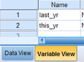
3.5.1 Define Your Variables
First, click the “Variable View” tab at the bottom of your screen. Then, type the names of your variables in the “Name” column. As shown in Figure 3.2, we have named our variables “last_yr” and “this_yr.”
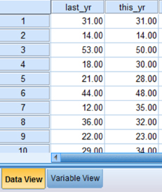
3.5.2 Type in Your Values
Click the “Data View” tab at the bottom of your screen and type your data under the variable names. As shown in Figure 3.3, we are comparing “last_yr” with “this_yr.”
3.5.3 Analyze Your Data
As shown in Figure 3.4, use the pull-down menus to choose “Analyze,” “Nonparametric Tests,” “Legacy Dialogs,” and “2 Related Samples…”

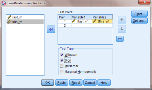
In the upper left box, select both variables that you want to compare. Then, use the arrow button to place your variable pair in the box labeled “Test Pairs:”. Next, check the “Test Type” you wish to perform. In Figure 3.5, we have checked “Wilcoxon” and “Sign” to perform both tests. Finally, click “OK” to perform the analysis.
3.5.4 Interpret the Results from the SPSS Output Window
SPSS Output 3.1 begins by reporting the results from the Wilcoxon signed rank test. The first output table (called “Ranks”) provides the Wilcoxon T or obtained value. From the “Sum of Ranks” column, we select the smaller of the two values. In our example, T = 7.5. The second output table (called “Test Statistics”) returns the critical z-score for large samples. In addition, SPSS calculates the two-tailed significance (p = 0.041).
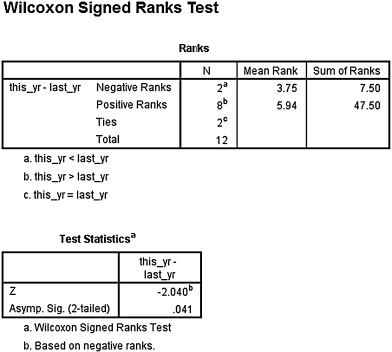
Based on the results from SPSS, the number of successful interventions was significantly different (T = 7.5, n = 12, p < 0.05). In addition, the sum of the positive difference ranks (ΣR+ = 47.5) was larger than the sum of the negative difference ranks (ΣR− = 7.5), demonstrating a positive impact from the program.
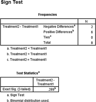
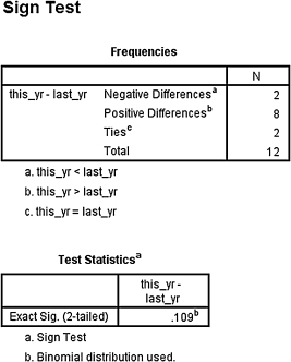
Next, SPSS Output 3.2 reports the results from the sign test. The first output table (called “Frequencies”) provides the negative differences, positive differences, ties, and total comparisons. The second output table (called “Test Statistics”) returns the two-tailed significance (p = 0.109). Based on the results of the sign test using SPSS, the number of successful interventions was not significantly different (0.109 > 0.05).
The notion that the Wilcoxon signed rank test produced significant results while the sign test did not is addressed next in a brief discussion about statistical power.
3.6 Statistical Power
Comparing our conflicting results from the small sample Wilcoxon signed rank test with the sign test presents an opportunity to discuss statistical power. That difference is especially visible when comparing the results from the sample problems in Sections 3.3.1 and 3.4.1 of this chapter. Both sections analyzed the same data; however, one section demonstrated a Wilcoxon signed rank test and the other demonstrated the sign test.
Notice that the result from the Wilcoxon signed rank test was significant, yet the result from the sign test was not significant. In other words, one test produced significant results and the other test did not. The reason involves differences in statistical power.
Nonparametric methods generally have less statistical power compared with their parametric equivalents, especially when used in small samples. For instance, a test with less statistical power has a smaller chance of detecting a true effect where one might actually exist. This difference in statistical power is especially true for the sign test (Siegel and Castellan, 1988).
A statistical test's power depends on several factors: the size of the effect (discussed later), level of desired significance (α), and sample size. Researchers use this information to perform a statistical power analysis before performing the experiment. This allows the researcher to determine the needed sample size. A quick search returns a variety of online power analysis tools. Currently, G*Power is a free tool. In addition, Cohen (1988) has provided several tables for finding sample sizes based on level of power.
3.7 Examples from the Literature
To be shown are varied examples of the nonparametric procedures described in this chapter. We have summarized each study's research problem and the researchers' rationale(s) for choosing a nonparametric approach. We encourage you to obtain these studies if you are interested in their results.
Boser and Poppen (1978) sought to determine which verbal responses by teacher held the greatest potential for improving student–teacher relationships. The seven verbal responses were feelings, thoughts, motives, behaviors, encounter/encouragement, confrontation, and sharing. They used a Wilcoxon signed rank test to examine 101 9th-grader responses because the student participants rank ordered their responses.
Vaughn et al. (1999) investigated kindergarten teachers' perceptions of practices identified to improve outcomes for children with disabilities transitioning from prekindergarten to kindergarten. The researchers compared the paired ratings of teachers' desirability to employ the identified practices with feasibility using a Wilcoxon signed rank test. This nonparametric procedure was considered the most appropriate because the study's measure was a Likert-type scale (1 = low, 5 = high).
Rinderknecht and Smith (2004) used a 7-month nutrition intervention to improve the dietary self-efficacy of Native American children (5–10 years) and adolescents (11–18 years). Wilcoxon signed rank tests were used to determine whether fat and sugar intake changed significantly between pre- and postintervention among adolescents. The researchers chose nonparametric tests for their data that were not normally distributed.
Seiver and Hatfield (2002) asked environmental health professionals about their willingness to dine in certain restaurants based on the method and history of health code evaluations. A paired-sample sign test was used to determine which health code evaluation method and history that participants preferred. The researchers chose a nonparametric test since they administered questionnaires with rank ordered scales (0 = never, 10 = always).
3.8 Summary
Two samples that are paired, or related, may be compared using a nonparametric procedure called the Wilcoxon signed rank test or the sign test. The parametric equivalent to this test is known as the Student's t-test, t-test for matched pairs, or t-test for dependent samples.
In this chapter, we described how to perform and interpret a Wilcoxon signed rank test and a sign test, using both small samples and large samples. We also explained how to perform the procedure for both tests using SPSS. Finally, we offered varied examples of these nonparametric statistics from the literature. The next chapter will involve comparing two samples that are not related.
3.9 Practice Questions
1. A teacher wished to determine if providing a bilingual dictionary to students with limited English proficiency improves math test scores. A small class of students (n = 10) was selected. Students were given two math tests. Each test covered the same type of math content; however, students were provided a bilingual dictionary on the second test. The data in Table 3.10 represent the students' performance on each math test.
Use a one-tailed Wilcoxon signed rank test and a one-tailed sign test to determine which testing condition resulted in higher scores. Use α = 0.05. Report your findings.
2. A research study was done to investigate the influence of being alone at night on the human male heart rate. Ten men were sent into a wooded area, one at a time, at night, for 20 min. They had a heart monitor to record their pulse rate. The second night, the same men were sent into a similar wooded area accompanied by a companion. Their pulse rate was recorded again. The researcher wanted to see if having a companion would change their pulse rate. The median rates are reported in Table 3.11.
Use a two-tailed Wilcoxon signed rank test and a two-tailed sign test to determine which condition produced a higher pulse rate. Use α = 0.05. Report your findings.
3. A researcher conducts a pilot study to compare two treatments to help obese female teenagers lose weight. She tests each individual in two different treatment conditions. The data in Table 3.12 provide the number of pounds that each participant lost.
Use a two-tailed Wilcoxon signed rank test and a two-tailed sign test to determine which treatment resulted in greater weight loss. Use α = 0.05. Report your findings.
4. Twenty participants in an exercise program were measured on the number of sit-ups they could do before other physical exercise (first count) and the number they could do after they had done at least 45 min of other physical exercise (second count). Table 3.13 shows the results for 20 participants obtained during two separate physical exercise sessions. Determine the ES for a calculated z-score.
5. A school is trying to get more students to participate in activities that will make learning more desirable. Table 3.14 shows the number of activities that each of the 10 students in one class participated in last year before a new activity program was implemented and this year after it was implemented. Construct a 95% median confidence interval based on the Wilcoxon signed rank test to determine whether the new activity program had a significant positive effect on the student participation.
| Student | Math test without a bilingual dictionary | Math test with a bilingual dictionary |
|---|---|---|
| 1 | 30 | 39 |
| 2 | 56 | 46 |
| 3 | 48 | 37 |
| 4 | 47 | 44 |
| 5 | 43 | 32 |
| 6 | 45 | 39 |
| 7 | 36 | 41 |
| 8 | 44 | 40 |
| 9 | 44 | 38 |
| 10 | 40 | 46 |
| Participant | Median rate alone | Median rate with companion |
|---|---|---|
| A | 88 | 72 |
| B | 77 | 74 |
| C | 91 | 80 |
| D | 70 | 77 |
| E | 80 | 71 |
| F | 85 | 83 |
| G | 90 | 80 |
| H | 82 | 91 |
| I | 93 | 86 |
| J | 75 | 69 |
| Participant | Pounds lost | |
|---|---|---|
| Treatment 1 | Treatment 2 | |
| 1 | 10 | 18 |
| 2 | 20 | 12 |
| 3 | 15 | 16 |
| 4 | 9 | 7 |
| 5 | 18 | 21 |
| 6 | 11 | 17 |
| 7 | 6 | 13 |
| 8 | 12 | 14 |
| Participant | First count | Second count |
|---|---|---|
| 1 | 18 | 28 |
| 2 | 19 | 18 |
| 3 | 20 | 28 |
| 4 | 29 | 20 |
| 5 | 15 | 30 |
| 6 | 22 | 25 |
| 7 | 21 | 28 |
| 8 | 30 | 18 |
| 9 | 22 | 27 |
| 10 | 11 | 30 |
| 11 | 20 | 24 |
| 12 | 21 | 27 |
| 13 | 21 | 10 |
| 14 | 20 | 40 |
| 15 | 18 | 20 |
| 16 | 27 | 14 |
| 17 | 24 | 29 |
| 18 | 13 | 30 |
| 19 | 10 | 24 |
| 20 | 10 | 36 |
| Participants | Last year | This year |
|---|---|---|
| 1 | 18 | 20 |
| 2 | 22 | 28 |
| 3 | 10 | 18 |
| 4 | 25 | 23 |
| 5 | 16 | 20 |
| 6 | 14 | 21 |
| 7 | 21 | 17 |
| 8 | 13 | 18 |
| 9 | 28 | 22 |
| 10 | 12 | 21 |
3.10 Solutions to Practice Questions
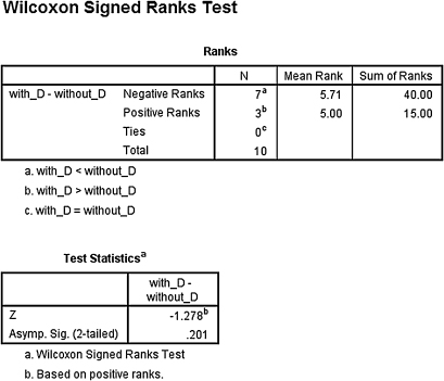
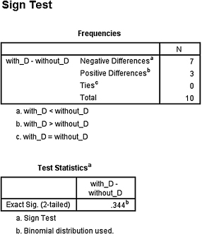
1. The results from the analysis are displayed in SPSS Outputs 3.3 and 3.4. Both tests report the two-tailed significance, but the question asked for the one-tailed significance. Therefore, divide the two-tailed significance by 2 to find the one-tailed significance.
The results from the Wilcoxon signed rank test reported a one-tailed significance of p = 0.201/2 = 0.101. The test results (T = 15.0, n = 10, p > 0.05) indicated that the two testing conditions were not significantly different.
The results from the sign test reported a one-tailed significance of p = 0.344/2 = 0.172. These test results (p > 0.05) also indicated that the two testing conditions were not significantly different.
Therefore, based on this study, the use of bilingual dictionaries on a math test did not significantly improve scores among limited English proficient students.
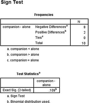
2. The results from the analysis are displayed in SPSS Outputs 3.5 and 3.6.
The results from the Wilcoxon signed rank test reported a two-tailed significance of p = 0.092. The test results (T = 11.0, n = 10, p > 0.05) indicated that the two conditions were not significantly different.
The results from the sign test reported a two-tailed significance of p = 0.109. These test results (p > 0.05) also indicated that the two testing conditions were not significantly different.
Therefore, based on this study, the presence of a companion in the woods at night did not significantly influence the males' pulse rates.
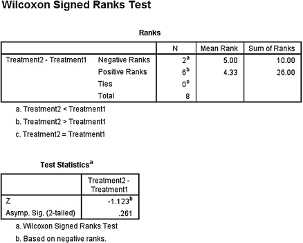
3. The results from the analysis are displayed in SPSS Outputs 3.7 and 3.8.
The results from the Wilcoxon signed rank test (T = 10.0, n = 8, p > 0.05) indicated that the two treatments were not significantly different.
The results from the sign test (p > 0.05) also indicated that the two testing conditions were not significantly different.
Therefore, based on this study, neither treatment program resulted in a significantly higher weight loss among obese female teenagers.
4. The results from the analysis are as follows:
This is a reasonably high ES which indicates a strong measure of association.
5. For our example, n = 10 and p = 0.05/2. Thus, T = 8 and K = 9. The ninth value from the bottom is −1.0 and the ninth value from the top is 7.0. Based on these findings, it is estimated with 95% confidence that the difference in students' number of activities before and after the new program lies between −1.0 and 7.0.