CHAPTER 4
Comparing Two Unrelated Samples: The Mann−Whitney U-Test and the Kolmogorov−Smirnov Two-Sample Test
4.1 Objectives
In this chapter, you will learn the following items:
- How to perform the Mann−Whitney U-test.
- How to construct a median confidence interval based on the difference between two independent samples.
- How to perform the Kolmogorov−Smirnov two-sample test.
- How to perform the Mann−Whitney U-test and the Kolmogorov−Smirnov two-sample test using SPSS®.
4.2 Introduction
Suppose a teacher wants to know if his first-period's early class time has been reducing student performance. To test his idea, he compares the final exam scores of students in his first-period class with those in his fourth-period class. In this example, each score from one class period is independent, or unrelated, to the other class period.
The Mann−Whitney U-test and the Kolmogorov−Smirnov two-sample test are nonparametric statistical procedures for comparing two samples that are independent, or not related. The parametric equivalent to these tests is the t-test for independent samples.
In this chapter, we will describe how to perform and interpret a Mann−Whitney U-test and a Kolmogorov−Smirnov two-sample test. We will demonstrate both small samples and large samples for each test. We will also explain how to perform the procedure using SPSS. Finally, we offer varied examples of these nonparametric statistics from the literature.
4.3 Computing the Mann−Whitney U-Test Statistic
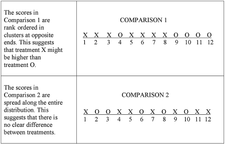
The Mann−Whitney U-test is used to compare two unrelated, or independent, samples. The two samples are combined and rank ordered together. The strategy is to determine if the values from the two samples are randomly mixed in the rank ordering or if they are clustered at opposite ends when combined. A random rank ordered would mean that the two samples are not different, while a cluster of one sample's values would indicate a difference between them. In Figure 4.1, two sample comparisons illustrate this concept.
Use Formula 4.1 to determine a Mann−Whitney U-test statistic for each of the two samples. The smaller of the two U statistics is the obtained value:
where Ui is the test statistic for the sample of interest, ni is the number of values from the sample of interest, n1 is the number of values from the first sample, n2 is the number of values from the second sample, and ΣRi is the sum of the ranks from the sample of interest.
After the U statistic is computed, it must be examined for significance. We may use a table of critical values (see Table B.4 in Appendix B). However, if the numbers of values in each sample, ni, exceeds those available from the table, then a large sample approximation may be performed. For large samples, compute a z-score and use a table with the normal distribution (see Table B.1 in Appendix B) to obtain a critical region of z-scores. Formula 4.2, Formula 4.3, and Formula 4.4 are used to find the z-score of a Mann−Whitney U-test for large samples:
where ![]() is the mean, n1 is the number of values from the first sample, and n2 is the number of values from the second sample;
is the mean, n1 is the number of values from the first sample, and n2 is the number of values from the second sample;
where sU is the standard deviation;
where z* is the z-score for a normal approximation of the data and Ui is the U statistic from the sample of interest.
At this point, the analysis is limited to identifying the presence or absence of a significant difference between the groups and does not describe the strength of the treatment. We can consider the effect size (ES) to determine the degree of association between the groups. We use Formula 4.5 to calculate the ES:
where |z| is the absolute value of the z-score and n is the total number of observations.
The ES ranges from 0 to 1. Cohen (1988) defined the conventions for ES as small = 0.10, medium = 0.30, and large = 0.50. (Correlation coefficient and ES are both measures of association. See Chapter 7 concerning correlation for more information on Cohen's assignment of ES's relative strength.)
4.3.1 Sample Mann−Whitney U-Test (Small Data Samples)
The following data were collected from a study comparing two methods being used to teach reading recovery in the 4th grade. Method 1 was a pull-out program in which the children were taken out of the classroom for 30 min a day, 4 days a week. Method 2 was a small group program in which children were taught in groups of four or five for 45 min a day in the classroom, 4 days a week. The students were tested using a reading comprehension test after 4 weeks of the program. The test results are shown in Table 4.1.
| Method 1 | Method 2 |
|---|---|
| 48 | 14 |
| 40 | 18 |
| 39 | 20 |
| 50 | 10 |
| 41 | 12 |
| 38 | 102 |
| 53 | 17 |
4.3.1.1 State the Null and Research Hypotheses
The null hypothesis states that there is no tendency of the ranks of one method to be systematically higher or lower than the other. The hypothesis is stated in terms of comparison of distributions, not means. The research hypothesis states that the ranks of one method are systematically higher or lower than the other. Our research hypothesis is a two-tailed, nondirectional hypothesis because it indicates a difference, but in no particular direction.
The null hypothesis is
HO: There is no tendency for ranks of one method to be significantly higher (or lower) than the other.
The research hypothesis is
HA: The ranks of one method are systematically higher (or lower) than the other.
4.3.1.2 Set the Level of Risk (or the Level of Significance) Associated with the Null Hypothesis
The level of risk, also called an alpha (α), is frequently set at 0.05. We will use α = 0.05 in our example. In other words, there is a 95% chance that any observed statistical difference will be real and not due to chance.
4.3.1.3 Choose the Appropriate Test Statistic
The data are obtained from two independent, or unrelated, samples of 4th-grade children being taught reading. Both the small sample sizes and an existing outlier in the second sample violate our assumptions of normality. Since we are comparing two unrelated, or independent, samples, we will use the Mann−Whitney U-test.
4.3.1.4 Compute the Test Statistic
First, combine and rank both data samples together (see Table 4.2).
| Ordered scores | ||
|---|---|---|
| Rank | Score | Sample |
| 1 | 10 | Method 2 |
| 2 | 12 | Method 2 |
| 3 | 14 | Method 2 |
| 4 | 17 | Method 2 |
| 5 | 18 | Method 2 |
| 6 | 20 | Method 2 |
| 7 | 38 | Method 1 |
| 8 | 39 | Method 1 |
| 9 | 40 | Method 1 |
| 10 | 41 | Method 1 |
| 11 | 48 | Method 1 |
| 12 | 50 | Method 1 |
| 13 | 53 | Method 1 |
| 14 | 102 | Method 2 |
Next, compute the sum of ranks for each method. Method 1 is ΣR1 and method 2 is ΣR2. Using Table 4.2,
and
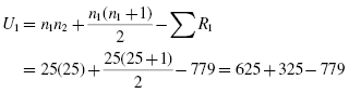
Now, compute the U-value for each sample. For sample 1,
and for sample 2,
The Mann−Whitney U-test statistic is the smaller of U1 and U2. Therefore, U = 7.
4.3.1.5 Determine the Value Needed for Rejection of the Null Hypothesis Using the Appropriate Table of Critical Values for the Particular Statistic
Since the sample sizes are small (n < 20), we use Table B.4 in Appendix B, which lists the critical values for the Mann−Whitney U. The critical values are found on the table at the point for n1 = 7 and n2 = 7. We set α = 0.05. The critical value for the Mann−Whitney U is 8. A calculated value that is less than or equal to 8 will lead us to reject our null hypothesis.
4.3.1.6 Compare the Obtained Value with the Critical Value
The critical value for rejecting the null hypothesis is 8 and the obtained value is U = 7. If the critical value equals or exceeds the obtained value, we must reject the null hypothesis. If instead, the critical value is less than the obtained value, we must not reject the null hypothesis. Since the critical value exceeds the obtained value, we must reject the null hypothesis.
4.3.1.7 Interpret the Results
We rejected the null hypothesis, suggesting that a real difference exists between the two methods. In addition, since the sum of the ranks for method 1 (ΣR1) was larger than method 2 (ΣR2), we see that method 1 had significantly higher scores.
4.3.1.8 Reporting the Results
The reporting of results for the Mann−Whitney U-test should include such information as the sample sizes for each group, the U statistic, the p-value's relation to α, and the sums of ranks for each group.
For this example, two methods were used to provide students with reading instruction. Method 1 involved a pull-out program and method 2 involved a small group program. Using the ranked reading comprehension test scores, the results indicated a significant difference between the two methods (U = 7, n1 = 7, n2 = 7, p < 0.05). The sum of ranks for method 1 (ΣR1 = 70) was larger than the sum of ranks for method 2 (ΣR2 = 35). Therefore, we can state that the data support the pull-out program as a more effective reading program for teaching comprehension to 4th-grade children at this school.
4.3.2 Confidence Interval for the Difference between Two Location Parameters
The American Psychological Association (2001) has suggested that researchers report the confidence interval for research data. A confidence interval is an inference to a population in terms of an estimation of sampling error. More specifically, it provides a range of values that fall within the population with a level of confidence of 100(1 − α)%.
A median confidence interval can be constructed based on the difference between two independent samples. It consists of possible values of differences for which we do not reject the null hypothesis at a defined significance level of α.
The test depends on the following assumptions:
- Data consist of two independent random samples: X1, X2, … , Xn from one population and Y1, Y2, … , Yn from the second population.
- The distribution functions of the two populations are identical except for possible location parameters.
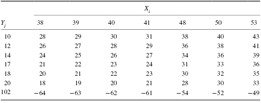
To perform the analysis, set up a table that identifies all possible differences for each possible sample pair such that Dij = Xi − Yj for (Xi,Yj). Placing the values for X from smallest to largest across the top and the values for Y from smallest to largest down the side will eliminate the need to order the values of Dij later.
The sample procedure to be presented later is based on the data from Table 4.2 (small data sample Mann−Whitney U-test) near the beginning of this chapter.
The values from Table 4.2 are arranged in Table 4.3 so that the method 1 (X) scores are placed in order across the top and the method 2 (Y) scores are placed in order down the side. Then, the n1n2 differences are calculated by subtracting each Y value from each X value. The differences are shown in Table 4.3. Notice that the values of Dij are ordered in the table from highest to lowest starting at the top right and ending at the bottom left.
We use Table B.4 in Appendix B to find the lower limit of the confidence interval, L, and the upper limit U. For a two-tailed test, L is the wα/2th smallest difference and U is the wα/2th largest difference that correspond to α/2 for n1 and n2 for a confidence interval of (1 − α).
For our example, n1 = 7 and n2 = 7. For α/2 = 0.05/2 = 0.025, Table B.4 returns wα/2 = 9. This means that the ninth values from the top and bottom mark the limits of the 95% confidence interval on both ends. Therefore, L = 19 and U = 36. Based on these results, we are 95% certain that the difference in population median is between 18 and 36.
4.3.3 Sample Mann−Whitney U-Test (Large Data Samples)
The previous comparison of teaching methods for reading recovery was repeated with 5th-grade students. The 5th-grade used the same two methods. Method 1 was a pull-out program in which the children were taken out of the classroom for 30 min a day, 4 days a week. Method 2 was a small group program in which children were taught in groups of four or five for 45 min a day in the classroom, 4 days a week. The students were tested using the same reading comprehension test after 4 weeks of the program. The test results are shown in Table 4.4.
| Method 1 | Method 2 |
|---|---|
| 48 | 14 |
| 40 | 18 |
| 39 | 20 |
| 50 | 10 |
| 41 | 12 |
| 38 | 102 |
| 71 | 21 |
| 30 | 19 |
| 15 | 100 |
| 33 | 23 |
| 47 | 16 |
| 51 | 82 |
| 60 | 13 |
| 59 | 25 |
| 58 | 24 |
| 42 | 97 |
| 11 | 28 |
| 46 | 9 |
| 36 | 34 |
| 27 | 52 |
| 93 | 70 |
| 72 | 22 |
| 57 | 26 |
| 45 | 8 |
| 53 | 17 |
4.3.3.1 State the Null and Research Hypotheses
The null hypothesis states that there is no tendency of the ranks of one method to be systematically higher or lower than the other. The hypothesis is stated in terms of comparison of distributions, not means. The research hypothesis states that the ranks of one method are systematically higher or lower than the other. Our research hypothesis is a two-tailed, nondirectional hypothesis because it indicates a difference, but in no particular direction.
The null hypothesis is
HO: There is no tendency for ranks of one method to be significantly higher (or lower) than the other.
The research hypothesis is
HA: The ranks of one method are systematically higher (or lower) than the other.
4.3.3.2 Set the Level of Risk (or the Level of Significance) Associated with the Null Hypothesis
The level of risk, also called an alpha (α), is frequently set at 0.05. We will use α = 0.05 in our example. In other words, there is a 95% chance that any observed statistical difference will be real and not due to chance.
4.3.3.3 Choose the Appropriate Test Statistic
The data are obtained from two independent, or unrelated, samples of 5th-grade children being taught reading. Since we are comparing two unrelated, or independent, samples, we will use the Mann−Whitney U-test.
4.3.3.4 Compute the Test Statistic
First, combine and rank both data samples together (see Table 4.5). Next, compute the sum of ranks for each method. Method 1 is ΣR1 and method 2 is ΣR2. Using Table 4.5,
| Ordered scores | ||
|---|---|---|
| Rank | Score | Sample |
| 1 | 8 | Method 2 |
| 2 | 9 | Method 2 |
| 3 | 10 | Method 2 |
| 4 | 11 | Method 1 |
| 5 | 12 | Method 2 |
| 6 | 13 | Method 2 |
| 7 | 14 | Method 2 |
| 8 | 15 | Method 1 |
| 9 | 16 | Method 2 |
| 10 | 17 | Method 2 |
| 11 | 18 | Method 2 |
| 12 | 19 | Method 2 |
| 13 | 20 | Method 2 |
| 14 | 21 | Method 2 |
| 15 | 22 | Method 2 |
| 16 | 23 | Method 2 |
| 17 | 24 | Method 2 |
| 18 | 25 | Method 2 |
| 19 | 26 | Method 2 |
| 20 | 27 | Method 1 |
| 21 | 28 | Method 2 |
| 22 | 30 | Method 1 |
| 23 | 33 | Method 1 |
| 24 | 34 | Method 2 |
| 25 | 36 | Method 1 |
| 26 | 38 | Method 1 |
| 27 | 39 | Method 1 |
| 28 | 40 | Method 1 |
| 29 | 41 | Method 1 |
| 30 | 42 | Method 1 |
| 31 | 45 | Method 1 |
| 32 | 46 | Method 1 |
| 33 | 47 | Method 1 |
| 34 | 48 | Method 1 |
| 35 | 50 | Method 1 |
| 36 | 51 | Method 1 |
| 37 | 52 | Method 2 |
| 38 | 53 | Method 1 |
| 39 | 57 | Method 1 |
| 40 | 58 | Method 1 |
| 41 | 59 | Method 1 |
| 42 | 60 | Method 1 |
| 43 | 70 | Method 2 |
| 44 | 71 | Method 1 |
| 45 | 72 | Method 1 |
| 46 | 82 | Method 2 |
| 47 | 93 | Method 1 |
| 48 | 97 | Method 2 |
| 49 | 100 | Method 2 |
| 50 | 102 | Method 2 |
and
Now, compute the U-value for each sample. For sample 1,
and for sample 2,
The Mann−Whitney U-test statistic is the smaller of U1 and U2. Therefore, U = 171.
Since our sample sizes are large, we will approximate them to a normal distribution. Therefore, we will find a z-score for our data using a normal approximation. We must find the mean ![]() and the standard deviation sU for the data:
and the standard deviation sU for the data:
and
Next, we use the mean, standard deviation, and the U-test statistic to calculate a z-score. Remember, we are testing the hypothesis that there is no difference in the ranks of the scores for two different methods of reading instruction for 5th-grade students:
4.3.3.5 Determine the Value Needed for Rejection of the Null Hypothesis Using the Appropriate Table of Critical Values for the Particular Statistic
Table B.1 in Appendix B is used to establish the critical region of z-scores. For a two-tailed test with α = 0.05, we must not reject the null hypothesis if −1.96 ≤ z* ≤ 1.96.
4.3.3.6 Compare the Obtained Value with the Critical Value
We find that z* is not within the critical region of the distribution, −2.75 < −1.96. Therefore, we reject the null hypothesis. This suggests a difference between method 1 and method 2.
4.3.3.7 Interpret the Results
We rejected the null hypothesis, suggesting that a real difference exists between the two methods. In addition, since the sum of the ranks for method 1 (ΣR1) was larger than method 2 (ΣR2), we see that method 1 had significantly higher scores.
At this point, the analysis is limited to identifying the presence or absence of a significant difference between the groups. In other words, the statistical test's level of significance does not describe the strength of the treatment. The American Psychological Association (2001), however, has called for a measure of the strength called the effect size.
We can consider the ES for this large sample test to determine the degree of association between the groups. We can use Formula 4.5 to calculate the ES. For the example, z = −2.75 and n = 50:
Our ES for the sample difference is 0.39. This value indicates a medium−high level of association between the teaching methods for the reading recovery program with 5th graders.
4.3.3.8 Reporting the Results
For this example, two methods were used to provide 5th-grade students with reading instruction. Method 1 involved a pull-out program and method 2 involved a small group program. Using the ranked reading comprehension test scores, the results indicated a significant difference between the two methods (U = 171, n1 = 25, n2 = 25, p < 0.05). The sum of ranks for method 1 (ΣR1 = 779) was larger than the sum of ranks for method 2 (ΣR2 = 496). Moreover, the ES for the sample difference was 0.39. Therefore, we can state that the data support the pull-out program as a more effective reading program for teaching comprehension to 5th-grade children at this school.
4.4 Computing the Kolmogorov–Smirnov Two-Sample Test Statistic
In Chapter 2, we used the Kolmogorov–Smirnov one-sample test to compare a sample with the normal distribution. We can use the Kolmogorov–Smirnov two-sample test to analyze two different data samples for independence. Our data must meet two assumptions.
- Observations X1, … , Xm are a random sample from a continuous population 1, where the X-values are mutually independent and identically distributed. Likewise, observations Y1, … , Yn are a random sample from a continuous population 2, where the Y-values are mutually independent and identically distributed.
- The two samples are independent.
We begin by placing the data in a form that will permit us to compute the two-sided Kolmogorov–Smirnov test statistic Z. The first step in this procedure is to find the empirical distribution functions Fm(t) and Gn(t) for the samples of X and Y, respectively. Combine and rank order both sets of values. For every real number t, let
and
where m is the sample size of X and n the sample size of Y.
Next, use Formula 4.6 to find each absolute value divergence D between the empirical distributions functions:
Use the largest divergence Dmax with Formula 4.7 to calculate the Kolmogorov–Smirnov test statistic Z:
Then, use the Kolmogorov–Smirnov test statistic, Z, and the Smirnov (1948) formula (see Formula 4.8, Formula 4.9, Formula 4.10, Formula 4.11, Formula 4.12, and Formula 4.13) to find the two-tailed probability estimate p. This is the same procedure shown in Chapter 2 when we performed the Kolmogorov–Smirnov one-sample test:
where
where
Once we have our p-value, we can compare it against our level of risk α to determine if the two samples are significantly different.
4.4.1 Sample Kolmogorov–Smirnov Two-Sample Test
We will use the data from Section 4.3.1 to demonstrate the Kolmogorov–Smirnov two-sample test. Table 4.6 recalls the data from the study involving reading recovery in the 4th grade. Method 1 was a program in which children were taken out of the classroom for 30 min a day, Monday through Thursday each week. Method 2 was a small group program in which the children were taught in groups of no more than five for 45 min a day in the classroom. These small classes were taught Monday through Thursday, also. The students were tested using a reading comprehension test after 4 weeks of instruction.
| Method 1 | Method 2 |
|---|---|
| 48 | 14 |
| 40 | 18 |
| 39 | 20 |
| 50 | 10 |
| 41 | 12 |
| 38 | 102 |
| 53 | 17 |
4.4.1.1 State the Null and Alternate Hypotheses
Let X1, … , Xm, and Y1, … , Yn be independent random samples. The null hypothesis indicates that there is no difference between the reading groups X and Y. Our research hypothesis is a two-tailed, nondirectional hypothesis because it indicates a difference, but in no particular direction.
The null hypothesis is
HO: [F(t) = G(t), for every t]
The research hypothesis is
HA: [F(t) ≠ G(t) for at least one value of t]
4.4.1.2 Set the Level of Risk (or the Level of Significance) Associated with the Null Hypothesis
We will use α = 0.05 in our example. In other words, there is a 95% chance that any observed statistical difference will be real and not due to chance.
4.4.1.3 Choose the Appropriate Test Statistic
We are seeking to compare two random samples, X and Y. Each sample is mutually independent and identically distributed. The X's and Y's are mutually independent. The Kolmogorov–Smirnov two-sample test will provide this comparison.
4.4.1.4 Compute the Test Statistic
Begin by computing the empirical distribution functions for the X and Y samples:
and
where m = 7 and n = 7.
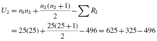
We use the data in Table 4.6 and Formula 4.6 to find each divergence and generate Table 4.7.
Next, we find the largest divergence Dmax. Table 4.7 shows that Dmax = 6/7 = 0.86. Now, we use Formula 4.7 to calculate the Kolmogorov–Smirnov test statistic Z:
4.4.1.5 Determine the p-Value Associated with the Test Statistic
Now, we find the p-value using Formula 4.11 since they satisfy the condition that 1 ≤ Z < 3.1. We first need Q using Formula 4.12:
Now, we can use Formula 4.11:
4.4.1.6 Compare the Obtained Value with the Critical Value Needed for Rejection of the Null Hypothesis
The two-tailed probability, p = 0.012, was computed and is now compared with the level of risk specified earlier, α = 0.05. If α is greater than the p-value, we must reject the null hypothesis. If α is less than the p-value, we must not reject the null hypothesis. Since α is greater than the p-value (0.05 > 0.012), we reject the null hypothesis.
4.4.1.7 Interpret the Results
We rejected the null hypothesis, suggesting that the two methods for teaching reading recovery have significantly different effects on the learning of students. In studying the results, it appears that method 1 was more effective than method 2, in general.
4.4.1.8 Reporting the Results
When reporting the results from the Kolmogorov–Smirnov two-sample test, include such information as the sample sizes for each group, the D statistic, and the p-value's relation to α.
For this example, two methods were used to provide students with reading instruction. Method 1 involved a pull-out program and method 2 involved a small group program. Both methods include seven participants. The results from the Kolmogorov–Smirnov two-sample test (D = 0.857, p < 0.05) indicate a significant difference between the two methods. Therefore, we can state that the data support the pull-out program as a more effective reading program for teaching comprehension to 4th-grade children at this school.
4.5 Performing the Mann–Whitney U-Test and the Kolmogorov–Smirnov Two-Sample Test Using SPSS
We will analyze the data from the example in Sections 4.3.1 and 4.4.1 using SPSS.
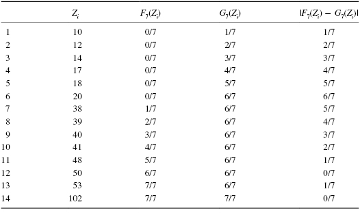
4.5.1 Define Your Variables
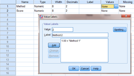
First, click the “Variable View” tab at the bottom of your screen. Then, type the names of your variables in the “Name” column. Unlike the related samples described in Chapter 2, you cannot simply enter each unrelated samples into a separate column to execute the Mann–Whitney U-test or Kolmogorov–Smirnov two-sample test. You must use a grouping variable to distinguish each sample. As shown in Figure 4.2, the first variable is the grouping variable that we called “Method.” The second variable that we called “Score” will have our actual values.
When establishing a grouping variable, it is often easiest to assign each group a whole number value. In our example, our groups are “Method 1” and “Method 2.” Therefore, we must set our grouping variables for the variable “Method.” First, we selected the “Values” column and clicked the gray square, as shown in Figure 4.3. Then, we set a value of 1 to equal “Method 1.” Now, as soon as we click the “Add” button, we will have set “Method 2” equal to 2 based on the values we inserted above.
4.5.2 Type in Your Values
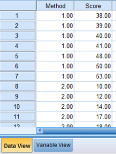
Click the “Data View” tab at the bottom of your screen as shown in Figure 4.4. Type in the values for both sets of data in the “Score” column. As you do so, type in the corresponding grouping variable in the “Method” column. For example, all of the values for “Method 2” are signified by a value of 2 in the grouping variable column that we called “Method.”
4.5.3 Analyze Your Data
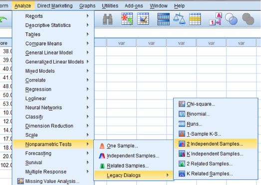
As shown in Figure 4.5, use the pull-down menus to choose “Analyze,” “Nonparametric Tests,” “Legacy Dialogs,” and “2 Independent Samples. …”
Use the top arrow button to place your variable with your data values, or dependent variable (DV), in the box labeled “Test Variable List:.” Then, use the lower arrow button to place your grouping variable, or independent variable (IV), in the box labeled “Grouping Variable.” As shown in Figure 4.6, we have placed the “Score” variable in the “Test Variable List” and the “Method” variable in the “Grouping Variable” box. Click on the “Define Groups …” button to assign a reference value to your IV (i.e., “Grouping Variable”).
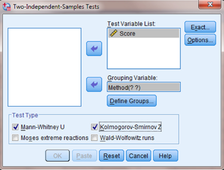
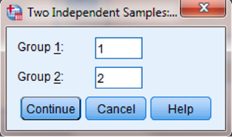
As shown in Figure 4.7, type 1 into the box next to “Group 1:” and 2 in the box next to “Group 2:.” Then, click “Continue.” This step references the value labels you created when you defined your grouping variable in step 1. Now that the groups have been assigned, click “OK” to perform the analysis.
4.5.4 Interpret the Results from the SPSS Output Window
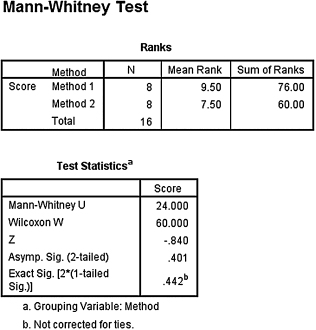
We first compare the samples with the Mann–Whitney U-test. SPSS Output 4.1 provides the sum of ranks and sample sizes for comparing the two groups. The second output table provides the Mann–Whitney U-test statistic (U = 7.0). As described in Figure 4.2, it also returns a similar nonparametric statistic called the Wilcoxon W-test statistic (W = 35.0). Notice that the Wilcoxon W is the smaller of the two rank sums in the table earlier.
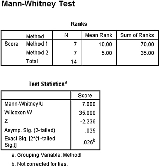
SPSS returns the critical z-score for large samples. In addition, SPSS calculates the two-tailed significance using two methods. The asymptotic significance is more appropriate with large samples. However, the exact significance is more appropriate with small samples or data that do not resemble a normal distribution.
Based on the results from SPSS, the ranked reading comprehension test scores of the two methods were significantly different (U = 7, n1 = 7, n2 = 7, p < 0.05). The sum of ranks for method 1 (ΣR1 = 70) was larger than the sum of ranks for method 2 (ΣR2 = 35).
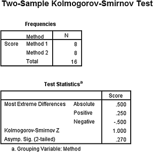
Next, we analyzed the data with the Kolmogorov–Smirnov two-sample test. SPSS Output 4.2 provides the most extreme differences, Dmax = 0.857. The second output table provides the Kolmogorov–Smirnov two-sample test statistic, Z = 1.604, and the two-tailed significance, p = 0.012.

The results from the Kolmogorov–Smirnov two-sample test (D = 0.857, p < 0.05) indicate a significant difference between the two methods. Therefore, we can state that the data support the pull-out program as a more effective reading program for teaching comprehension to 4th-grade children at this school.
4.6 Examples from the Literature
Listed are varied examples of the nonparametric procedures described in this chapter. We have summarized each study's research problem and researchers' rationale(s) for choosing a nonparametric approach. We encourage you to obtain these studies if you are interested in their results.
Odaci (2007) investigated depression, submissive social behaviors, and frequency of automatic negative thoughts in Turkish adolescents. Obese participants were compared with participants of normal weight. After the Shapiro–Wilk statistic revealed that the data were not normally distributed, Odaci applied a Mann–Whitney U-test to compare the groups.
Bryant and Trockel (1976) investigated the impact of stressful life events on undergraduate females' locus of control. The authors compared accrued life changing units for participants with internal control against external using the Mann–Whitney U-test. This nonparametric procedure was selected since the data pertaining to stressful life events were ordinal in nature.
Re et al. (2007) investigated the expressive writing of children with attention-deficit/hyperactivity disorder (ADHD). The authors used a Mann–Whitney U-test to compare students showing symptoms of ADHD behaviors with a control group of students not displaying such behaviors. After examining their data with a Kolmogorov–Smirnov test, the researchers chose the nonparametric procedure due to significant deviations in the data distributions.
In an effort to understand the factors that have motivated minority students to enter the social worker profession, Limb and Organista (2003) studied data from nearly 7000 students in California entering a social worker program. The authors used a Wilcoxon rank sum test to compare sums of student group ranks. They chose this nonparametric test due to a concern that statistical assumptions were violated regarding sample normality and homogeneity of variances.
Schulze and Tomal (2006) examined classroom climate perceptions among undergraduate students. Since the student questionnaires used an interval scale, they analyzed their findings with a Mann–Whitney U-test.
Hegedus (1999) performed a pilot study to evaluate a scale designed to examine the caring behaviors of nurses. Care providers were compared with the consumers. She used a Wilcoxon rank sum test in her analysis because study participants were directed to rank the items on the scale.
The nature of expertise in astronomy was investigated across a broad spectrum of ages and experience (Bryce and Blown 2012). For each age and experience level, the researchers compared groups in New Zealand with respective groups in China using several Kolmogorov–Smirnov two-sample tests. In other words, each set of the two independent samples were from New Zealand versus China. The researchers chose a nonparametric procedure since their data were categorized with an ordinal scale.
4.7 Summary
Two samples that are not related may be compared using a nonparametric procedure. Examples include the Mann–Whitney U-test (or the Wilcoxon rank sum test) and the Kolmogorov–Smirnov two-sample test. The parametric equivalent to these tests is known as the t-test for independent samples.
In this chapter, we described how to perform and interpret the Mann–Whitney U-test and the Kolmogorov–Smirnov two-sample test. We demonstrated both small samples and large samples for each test. We also explained how to perform the procedures using SPSS. Finally, we offered varied examples of these nonparametric statistics from the literature. The next chapter will involve comparing more than two samples that are related.
4.8 Practice Questions
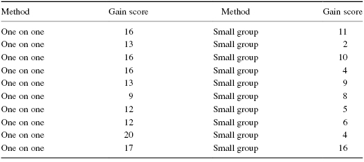
1. The data in Table 4.8 were obtained from a reading-level test for 1st-grade children. Compare the performance gains of the two different methods for teaching reading.
Use two-tailed Mann–Whitney U and Kolmogorov–Smirnov two-sample tests to determine which method was better for teaching reading. Set α = 0.05. Report your findings.
2. A research study was conducted to see if an active involvement in a hobby had a positive effect on the health of a person who retires after age 65. The data in Table 4.9 describe the health (number of doctor visits in 1 year) for participants who are involved in a hobby almost daily and those who are not.
Use one-tailed Mann–Whitney U and Kolmogorov–Smirnov two-sample tests to determine whether the hobby tends to reduce the need for doctor visits. Set α = 0.05. Report your findings.
3. Table 4.10 shows assessment scores of two different classes who are being taught computer skills using two different methods.
Use two-tailed Mann–Whitney U and Kolmogorov–Smirnov two-sample tests to determine which method was better for teaching computer skills. Set α = 0.05. Report your findings.
4. Two methods of teaching reading were compared. Method 1 used the computer to interact with the student, and diagnose and remediate the student based on misconceptions. Method 2 was taught using workbooks in classroom groups. Table 4.11 shows the data obtained on an assessment after 6 weeks of instruction. Calculate the ES using the z-score from the analysis.
5. Two methods were used to provide instruction in science for 7th grade. Method 1 included a laboratory each week and method 2 had only classroom work with lecture and worksheets. Table 4.12 shows end-of-course test performance for the two methods. Construct a 95% median confidence interval based on the difference between two independent samples to compare the two methods.
| No hobby group | Hobby group |
|---|---|
| 12 | 9 |
| 15 | 5 |
| 8 | 10 |
| 11 | 3 |
| 9 | 4 |
| 17 | 2 |
| Method 1 | Method 2 |
|---|---|
| 53 | 91 |
| 41 | 18 |
| 17 | 14 |
| 45 | 21 |
| 44 | 23 |
| 12 | 99 |
| 49 | 16 |
| 50 | 10 |
| Method 1 | Method 2 |
|---|---|
| 27 | 9 |
| 38 | 42 |
| 15 | 21 |
| 85 | 83 |
| 36 | 110 |
| 95 | 19 |
| 93 | 29 |
| 57 | 40 |
| 63 | 30 |
| 81 | 23 |
| 65 | 18 |
| 77 | 32 |
| 59 | 101 |
| 89 | 7 |
| 41 | 50 |
| 26 | 37 |
| 102 | 22 |
| 55 | 71 |
| 46 | 16 |
| 82 | 45 |
| 24 | 35 |
| 87 | 28 |
| 66 | 91 |
| 12 | 86 |
| 90 | 20 |
| Method 1 | Method 2 |
|---|---|
| 15 | 8 |
| 23 | 15 |
| 9 | 10 |
| 12 | 13 |
| 18 | 17 |
| 22 | 5 |
| 17 | 18 |
| 20 | 7 |
4.9 Solutions to Practice Questions
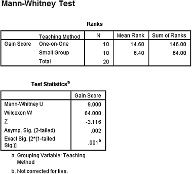
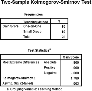
1. The results from the analysis are displayed in SPSS Outputs 4.3 and 4.4.
The results from the Mann–Whitney U-test (U = 9, n1 = 10, n2 = 10, p < 0.05) indicated that the two methods were significantly different. Moreover, the one-on-one method produced a higher sum of ranks (ΣR1 = 146) than the small group method (ΣR2 = 64).
The results from the Kolmogorov–Smirnov two-sample test (D = 1.789, p < 0.05) also suggested that the two methods were significantly different.
Therefore, based on both statistical tests, 1st-grade children displayed significantly higher reading levels when taught with a one-on-one method.
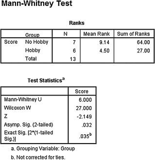
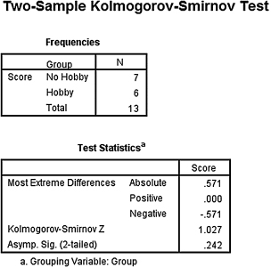
2. The results from the analysis are displayed in SPSS Outputs 4.5 and 4.6.
The results from the Mann–Whitney U-test (U = 6, n1 = 7, n2 = 6, p < 0.05) indicated that the two samples were significantly different. Moreover, the sample with no hobby produced a higher sum of ranks (ΣR1 = 64) than the sample with a hobby (ΣR2 = 27).
The results from the Kolmogorov–Smirnov two-sample test (D = 1.027, p > 0.05) suggested, however, that the two methods were not significantly different.
The conflicting results from the two statistical tests prevent us from making a conclusive statement about this study. Study replication with larger sample sizes is recommended.
3. The results from the analysis are displayed in SPSS Outputs 4.7 and 4.8.
The results from the Mann–Whitney U-test (U = 24, n1 = 8, n2 = 8, p > 0.05) and the results from the Kolmogorov–Smirnov two-sample test (D = 1.000, p > 0.05) indicated that the two samples were not significantly different. Therefore, based on this study, neither method resulted in significantly different assessment scores for computer skills.
4. The results from the analysis are as follows:
The ES is moderate.
5. For our example, n1 = 8 and n2 = 8. For 0.05/2 = 0.025, wα/2 = 14. Based on these results, we are 95% certain that the median difference between the two methods is between 0 and 11.