CHAPTER 8
Tests for Nominal Scale Data: Chi-Square and Fisher Exact Tests
8.1 Objectives
In this chapter, you will learn the following items:
- How to perform a chi-square goodness-of-fit test.
- How to perform a chi-square goodness-of-fit test using SPSS®.
- How to perform a chi-square test for independence.
- How to perform a chi-square test for independence using SPSS.
- How to perform the Fisher exact test.
- How to perform Fisher exact test using SPSS.
8.2 Introduction
Sometimes, data are best collected or conveyed nominally or categorically. These data are represented by counting the number of times a particular event or condition occurs. In such cases, you may be seeking to determine if a given set of counts, or frequencies, statistically matches some known, or expected, set. Or, you may wish to determine if two or more categories are statistically independent. In either case, we can use a nonparametric procedure to analyze nominal data.
In this chapter, we present three procedures for examining nominal data: chi-square (χ2) goodness of fit, χ2-test for independence, and the Fisher exact test. We will also explain how to perform the procedures using SPSS. Finally, we offer varied examples of these nonparametric statistics from the literature.
8.3 The χ2 Goodness-of-Fit Test
Some situations in research involve investigations and questions about relative frequencies and proportions for a distribution. Some examples might include a comparison of the number of women pediatricians with the number of men pediatricians, a search for significant changes in the proportion of students entering a writing contest over 5 years, or an analysis of customer preference of three candy bar choices. Each of these examples asks a question about a proportion in the population.
When comparing proportions, we are not measuring a numerical score for each individual. Instead, we classify each individual into a category. We then find out what proportion of the population is classified into each category. The χ2 goodness-of-fit test is designed to answer this type of question.
The χ2 goodness-of-fit test uses sample data to test the hypothesis about the proportions of the population distribution. The test determines how well the sample proportions fit the proportions specified in the null hypothesis.
8.3.1 Computing the χ2 Goodness-of-Fit Test Statistic
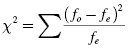
The χ2 goodness-of-fit test is used to determine how well the obtained sample proportions or frequencies for a distribution fit the population proportions or frequencies specified in the null hypothesis. The χ2 statistic can be used when two or more categories are involved in the comparison. Formula 8.1 is referred to as Pearson's χ2 and is used to determine the χ2 statistic:
where fo is the observed frequency (the data) and fe is the expected frequency (the hypothesis).
Use Formula 8.2 to determine the expected frequency fe:
where Pi is a category's frequency proportion with respect to the other categories and n is the sample size of all categories and ![]() .
.
Use Formula 8.3 to determine the degrees of freedom for the χ2-test:
where C is the number of categories.
8.3.2 Sample χ2 Goodness-of-Fit Test (Category Frequencies Equal)
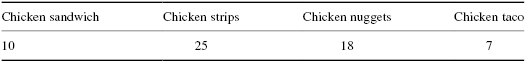
A marketing firm is conducting a study to determine if there is a significant preference for a type of chicken that is served as a fast food. The target group is college students. It is assumed that there is no preference when the study is started. The types of food that are being compared are chicken sandwich, chicken strips, chicken nuggets, and chicken taco.
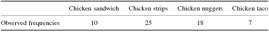
The sample size for this study was n = 60. The data in Table 8.1 represent the observed frequencies for the 60 participants who were surveyed at the fast food restaurants.
We want to determine if there is any preference for one of the four chicken fast foods that were purchased to eat by the college students. Since the data only need to be classified into categories, and no sample mean nor sum of squares needs to be calculated, the χ2 statistic goodness-of-fit test can be used to test the nonparametric data.
8.3.2.1 State the Null and Research Hypotheses
The null hypothesis states that there is no preference among the different categories. There is an equal proportion or frequency of participants selecting each type of fast food that uses chicken. The research hypothesis states that one or more of the chicken fast foods is preferred over the others by the college student.
The null hypothesis is
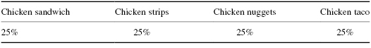
HO: In the population of college students, there is no preference of one chicken fast food over any other. Thus, the four fast food types are selected equally often and the population distribution has the proportions shown in Table 8.2.
HA: In the population of college students, there is at least one chicken fast food preferred over the others.
8.3.2.2 Set the Level of Risk (or the Level of Significance) Associated with the Null Hypothesis
The level of risk, also called an alpha (α), is frequently set at 0.05. We will use α = 0.05 in our example. In other words, there is a 95% chance that any observed statistical difference will be real and not due to chance.
8.3.2.3 Choose the Appropriate Test Statistic
The data are obtained from 60 college students who eat fast food chicken. Each student was asked which of the four chicken types of food he or she purchased to eat and the result was tallied under the corresponding category type. The final data consisted of frequencies for each of the four types of chicken fast foods. These categorical data, which are represented by frequencies or proportions, are analyzed using the χ2 goodness-of-fit test.
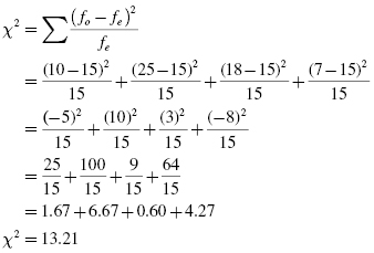
8.3.2.4 Compute the Test Statistic
First, tally the observed frequencies, fo, for the 60 students who were in the study. Use these data to create the observed frequency table shown in Table 8.3.
Next, calculate the expected frequency for each category. In this case, the expected frequency, fe, will be the same for all four categories since our research problem assumes that all categories are equal:
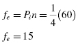
Table 8.4 presents the expected frequencies for each category.
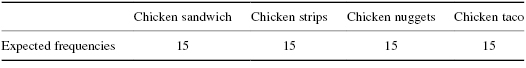
Using the values for the observed and expected frequencies, the χ2 statistic may be calculated:
8.3.2.5 Determine the Value Needed for Rejection of the Null Hypothesis Using the Appropriate Table of Critical Values for the Particular Statistic
Before we go to the table of critical values, we must determine the degrees of freedom, df. In this example, there are four categories, C = 4. To find the degrees of freedom, use df = C − 1 = 4 − 1. Therefore, df = 3.
Now, we use Table B.2 in Appendix B, which lists the critical values for the χ2. The critical value is found in the χ2 table for three degrees of freedom, df = 3. Since we set the α = 0.05, the critical value is 7.81. A calculated value that is greater than or equal to 7.81 will lead us to reject the null hypothesis.
8.3.2.6 Compare the Obtained Value with the Critical Value
The critical value for rejecting the null hypothesis is 7.81 and the obtained value is χ2 = 13.21. If the critical value is less than or equal to the obtained value, we must reject the null hypothesis. If instead, the critical value exceeds the obtained value, we do not reject the null hypothesis. Since the critical value is less than our obtained value, we must reject the null hypothesis.
Note that the critical value for α = 0.01 is 11.34. Since the obtained value is 13.21, a value greater than 11.34, the data indicate that the results are highly significant.
8.3.2.7 Interpret the Results
We rejected the null hypothesis, suggesting that there is a real difference among chicken fast food choices preferred by college students. In particular, the data show that a larger portion of the students preferred the chicken strips and only a few of them preferred the chicken taco.
8.3.2.8 Reporting the Results
The reporting of results for the χ2 goodness of fit should include such information as the total number of participants in the sample and the number that were classified in each category. In some cases, bar graphs are good methods of presenting the data. In addition, include the χ2 statistic, degrees of freedom, and p-value's relation to α. For this study, the number of students who ate each type of chicken fast food should be noted either in a table or plotted on a bar graph. The probability, p < 0.01, should also be indicated with the data to show the degree of significance of the χ2.
For this example, 60 college students were surveyed to determine which fast food type of chicken they purchased to eat. The four choices were chicken sandwich, chicken strips, chicken nuggets, and chicken taco. Student choices were 10, 25, 18, and 7, respectively. The χ2 goodness-of-fit test was significant (![]() , p < 0.01). Based on these results, a larger portion of the students preferred the chicken strips while only a few students preferred the chicken taco.
, p < 0.01). Based on these results, a larger portion of the students preferred the chicken strips while only a few students preferred the chicken taco.
8.3.3 Sample χ2 Goodness-of-Fit Test (Category Frequencies Not Equal)
Sometimes, research is being conducted in an area where there is a basis for different expected frequencies in each category. In this case, the null hypothesis will indicate different frequencies for each of the categories according to the expected values. These values are usually obtained from previous data that were collected in similar studies.
In this study, a school system uses three different physical fitness programs because of scheduling requirements. A researcher is studying the effect of the programs on 10th-grade students' 1-mile run performance. Three different physical fitness programs were used by the school system and will be described later.
- Program 1. Delivers health and physical education in 9-week segments with an alternating rotation of nine straight weeks of health education and then nine straight weeks of physical education.
- Program 2. Delivers health and physical education everyday with 30 min for health, 10 min for dress-out time, and 50 min of actual physical activity
- Program 3. Delivers health and physical education in 1-week segments with an alternating rotation of 1 week of health education and then 1 week of physical education
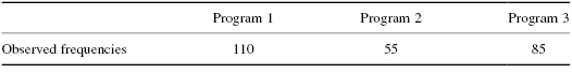
Using students who participated in all three programs, the researcher is comparing these programs based on student performances on the 1-mile run. The researcher recorded the program in which each student received the most benefit. Two hundred fifty students had participated in all three programs. The results for all of the students are recorded in Table 8.5.
| Program 1 | Program 2 | Program 3 |
|---|---|---|
| 110 | 55 | 85 |
We want to determine if the frequency distribution in the case earlier is different from previous studies. Since the data only need to be classified into categories, and no sample mean or sum of squares needs to be calculated, the χ2 goodness-of-fit test can be used to test the nonparametric data.
8.3.3.1 State the Null and Research Hypotheses
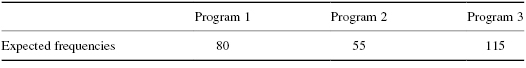
The null hypothesis states the proportion of students who benefited most from one of the three programs based on a previous study. As shown in Table 8.6, there are unequal expected frequencies for the null hypothesis. The research hypothesis states that there is at least one of the three categories that will have a different proportion or frequency than those identified in the null hypothesis.
| Program 1 | Program 2 | Program 3 |
|---|---|---|
| 32% | 22% | 45% |
The null hypothesis is
HO: The proportions do not differ from the previously determined proportions shown in Table 8.6.
HA: The population distribution has a different shape than that specified in the null hypothesis.
8.3.3.2 Set the Level of Risk (or the Level of Significance) Associated with the Null Hypothesis
The level of risk, also called an alpha (α), is frequently set at 0.05. We will use α = 0.05 in our example. In other words, there is a 95% chance that any observed statistical difference will be real and not due to chance.
8.3.3.3 Choose the Appropriate Test Statistic
The data are being obtained from the 1-mile run performance of 250 10th-grade students who participated in a school system's three health and physical education programs. Each student was categorized based on the plan in which he or she benefited most. The final data consisted of frequencies for each of the three plans. These categorical data which are represented by frequencies or proportions are analyzed using the χ2 goodness-of-fit test.
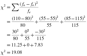
8.3.3.4 Compute the Test Statistic
First, tally the observed frequencies for the 250 students who were in the study. This was performed by the researcher. Use the data to create the observed frequency table shown in Table 8.7.
Next, calculate the expected frequencies for each category. In this case, the expected frequency will be different for each category. Each one will be based on proportions stated in the null hypothesis:
Table 8.8 presents the expected frequencies for each category.
Use the values for the observed and expected frequencies calculated earlier to calculate the χ2 statistic:
8.3.3.5 Determine the Value Needed for Rejection of the Null Hypothesis Using the Appropriate Table of Critical Values for the Particular Statistic
Before we go to the table of critical values, we must determine the degrees of freedom, df. In this example, there are four categories, C = 3. To find the degrees of freedom, use df = C − 1 = 3 − 1. Therefore, df = 2.
Now, we use Table B.2 in Appendix B, which lists the critical values for the χ2. The critical value is found in the χ2 table for two degrees of freedom, df = 2. Since we set α = 0.05, the critical value is 5.99. A calculated value that is greater than 5.99 will lead us to reject the null hypothesis.
8.3.3.6 Compare the Obtained Value with the Critical Value
The critical value for rejecting the null hypothesis is 5.99 and the obtained value is χ2 = 19.08. If the critical value is less than or equal to the obtained value, we must reject the null hypothesis. If instead, the critical value exceeds the obtained value, we do not reject the null hypothesis. Since the critical value is less than our obtained value, we must reject the null hypothesis.
Note that the critical value for α = 0.01 is 9.21. Since the obtained value is 19.08, which is greater than the critical value, the data indicate that the results are highly significant.
8.3.3.7 Interpret the Results
We rejected the null hypothesis, suggesting that there is a real difference in how the health and physical education program affects the performance of students on the 1-mile run as compared with the existing research. By comparing the expected frequencies of the past study and those obtained in the current study, it can be noted that the results from program 2 did not change. Program 2 was least effective in both cases, with no difference between the two. Program 1 became more effective and program 3 became less effective.
8.3.3.8 Reporting the Results
The reporting of results for the χ2 goodness-of-fit should include such information as the total number of participants in the sample, the number that were classified in each category, and the expected frequencies that are being used for comparison. It is important also to cite a source for the expected frequencies so that the decisions made from the study can be supported. In addition, include the χ2 statistic, degrees of freedom, and p-value's relation to α. It is often a good idea to present a bar graph to display the observed and expected frequencies from the study. For this study, the probability, p < 0.01, should also be indicated with the data to show the degree of significance of the χ2.
For this example, 250 10th-grade students participated in three different health and physical education programs. Using 1-mile run performance, students' program of greatest benefit was compared with the results from past research. The χ2 goodness-of-fit test was significant (![]() , p < 0.01). Based on these results, program 2 was least effective in both cases, with no difference between the two. Program 1 became more effective and program 3 became less effective.
, p < 0.01). Based on these results, program 2 was least effective in both cases, with no difference between the two. Program 1 became more effective and program 3 became less effective.
8.3.4 Performing the χ2 Goodness-of-Fit Test Using SPSS
We will analyze the data from the example earlier using SPSS.
8.3.4.1 Define Your Variables
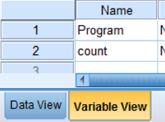
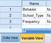
First, click the “Variable View” tab at the bottom of your screen (see Fig. 8.1). The χ2 goodness-of-fit test requires two variables: one variable to identify the categories and a second variable to identify the observed frequencies. Type the names of these variables in the “Name” column. In our example, we define the variables as “Program” and “count.”
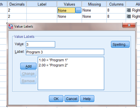
You must assign values to serve as a reference for each category in the observed frequency variable. It is often easiest to assign each category a whole number value. As shown in Figure 8.2, our categories are “Program 1,” “Program 2,” and “Program 3.” First, we selected the “count” variable and clicked the gray square in the “Values” field. Then, we set a value of 1 to equal “Program 1,” a value of 2 to equal “Program 2,” and a value of 3 to equal “Program 3.” We use the “Add” button to move the variable labels to the box below. Repeat this procedure for the “Program” variable so that the output tables will display these labels.
8.3.4.2 Type in Your Values
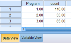
Click the “Data View” tab at the bottom of your screen. First, enter the data for each category using the whole numbers you assigned to represent the categories. As shown in Figure 8.3, we entered the values “1,” “2,” and “3” in the “Program” variable. Second, enter the observed frequencies next to the corresponding category values. In our example, we entered the observed frequencies “110,” “55,” and “85.”
8.3.4.3 Analyze Your Data
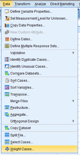
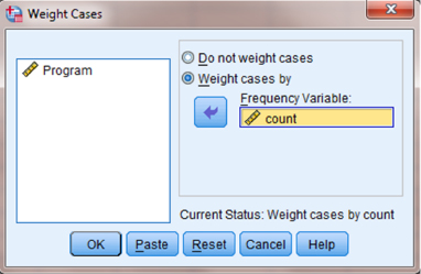
First, use the “Weight Cases” command to allow the observed frequency variable to reference the category variable. As shown in Figure 8.4, use the pull-down menus to choose “Data” and “Weight Cases …”.
The default setting is “Do not weight cases.” Click the circle next to “Weight cases by” as shown in Figure 8.5. Select the variable with the observed frequencies. Move that variable to the “Frequency Variable:” box by clicking the small arrow button. In our example, we have moved the “count” variable. Finally, click “OK.”
As shown in Figure 8.6, use the pull-down menus to choose “Analyze,” “Nonparametric Tests,” “Legacy Dialogs,” and “Chi-square…”.

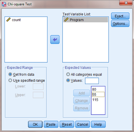
First, move the category variable to the “Test Variable List:” box by selecting that variable and clicking the small arrow button near the center of the window. As shown in Figure 8.7, we have chosen the “Program” variable. Then, enter your “Expected Values.” Notice that the option “All categories equal” is the default setting. Since this example does not have equal categories, we must select the “Values:” option to set the expected values. Enter the expected frequencies for each category in the order that they are listed in the SPSS Data View. After you type in an expected frequency in the “Values:” field, click “Add.” For our example, we have entered 80, 55, and 115, respectively. Finally, click “OK” to perform the analysis.
8.3.4.4 Interpret the Results from the SPSS Output Window
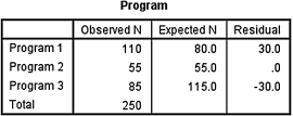
The first output table (see SPSS Output 8.1a) provides the observed and expected frequencies for each category and the total count.
The second output table (see SPSS Output 8.1b) provides the χ2 statistic (χ2 = 19.076), the degrees of freedom (df = 2), and the significance (p ≈ 0.000).
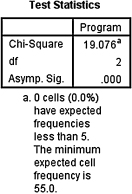
Based on the results from SPSS, three programs were compared with unequal expected frequencies. The χ2 goodness-of-fit test was significant (![]() , p < 0.01). Based on these results, program 2 was least effective in both cases, with no difference between the two. Program 1 became more effective and program 3 became less effective.
, p < 0.01). Based on these results, program 2 was least effective in both cases, with no difference between the two. Program 1 became more effective and program 3 became less effective.
8.4 The χ2 Test for Independence
Some research involves investigations of frequencies of statistical associations of two categorical attributes. Examples might include a sample of men and women who bought a pair of shoes or a shirt. The first attribute, A, is the gender of the shopper with two possible categories:
The second attribute, B, is the clothing type purchased by each individual:
We will assume that each person purchased only one item, either a pair of shoes or a shirt. The entire set of data is then arranged into a joint-frequency distribution table. Each individual is classified into one category which is identified by a pair of categorical attributes (see Table 8.9).
| A1 | A2 | |
|---|---|---|
| B1 | (A1, B1) | (A2, B1) |
| B2 | (A1, B2) | (A2, B2) |
The χ2-test for independence uses sample data to test the hypothesis that there is no statistical association between two categories. In this case, whether there is a significant association between the gender of the purchaser and the type of clothing purchased. The test determines how well the sample proportions fit the proportions specified in the null hypothesis.
8.4.1 Computing the χ2 Test for Independence
The χ2-test for independence is used to determine whether there is a statistical association between two categorical attributes. The χ2 statistic can be used when two or more categories are involved for two attributes. Formula 8.4 is referred to as Pearson's χ2 and is used to determine the χ2 statistic:
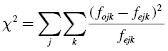
where fojk is the observed frequency for cell AjBk and fejk is the expected frequency for cell AjBk.
In tests for independence, the expected frequency fejk in any cell is found by multiplying the row total times the column total and dividing the product by the grand total N. Use Formula 8.5 to determine the expected frequency fejk:
The degrees of freedom df for the χ2 is found using Formula 8.6:
where R is the number of rows and C is the number of columns.
It is important to note that Pearson's χ2 formula returns a value that is too small when data form a 2 × 2 contingency table. This increases the chance of a type I error. In such a circumstance, one might use the Yates's continuity correction shown in Formula 8.7:
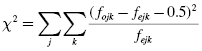
Daniel (1990) has cited a number of criticisms to the Yates's continuity correction. While he recognizes that the procedure has been frequently used, he also observes a decline in its popularity. Toward the end of this chapter, we present an alternative for analyzing a 2 × 2 contingency table using the Fisher exact test.
At this point, the analysis is limited to identifying an association's presence or absence. In other words, the χ2-test's level of significance does not describe the strength of its association. We can use the effect size to analyze the degree of association. For the χ2-test for independence, the effect size between the nominal variables of a 2 × 2 contingency table can be calculated and represented with the phi (ϕ) coefficient (see Formula 8.8):
where χ2 is the chi-square test statistic and n is the number in the entire sample.
The ϕ coefficient ranges from 0 to 1. Cohen (1988) defined the conventions for effect size as small = 0.10, medium = 0.30, and large = 0.50. (Correlation coefficient and effect size are both measures of association. See Chapter 7 concerning correlation for more information on Cohen's assignment of effect size's relative strength.)
When the χ2 contingency table is larger than 2 × 2, Cramer's V statistic may be used to express effect size. The formula for Cramer's V is shown in Formula 8.9:
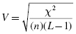
where χ2 is the chi-square test statistic, n is the total number in the sample, and L is the minimum value of the row totals and column totals from the contingency table.
8.4.2 Sample χ2 Test for Independence
A counseling department for a school system is conducting a study to investigate the association between children's attendance in public and private preschool and their behavior in the kindergarten classroom. It is the researcher's desire to see if there is any positive association between early exposure to learning and behavior in the classroom.
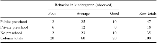
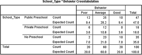
The sample size for this study was n = 100. The following data in Table 8.10 represent the observed frequencies for the 100 children whose behavior was observed during their first 6 weeks of school. The students who were in the study were identified by the type of preschool educational exposure they received.
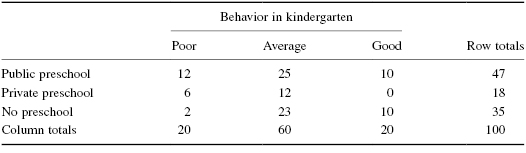
We want to determine if there is any association between type of preschool experience and behavior in kindergarten in the first 6 weeks of school. Since the data only need to be classified into categories, and no sample mean nor sum of squares needs to be calculated, the χ2 statistic for independence can be used to test the nonparametric data.
8.4.2.1 State the Null and Research Hypotheses
The null hypothesis states that there is no association between the two categories. The behavior of the children in kindergarten is independent of the type of preschool experience they had. The research hypothesis states that there is a significant association between the preschool experience of the children and their behavior in kindergarten.
The null hypothesis is
Ho: In the general population, there is no association between type of preschool experience a child has and the child's behavior in kindergarten.
The research hypothesis states
HA: In the general population, there is a predictable relationship between the preschool experience and the child's behavior in kindergarten.
8.4.2.2 Set the Level of Risk (or the Level of Significance) Associated with the Null Hypothesis
The level of risk, also called an alpha (α), is frequently set at 0.05. We will use α = 0.05 in our example. In other words, there is a 95% chance that any observed statistical difference will be real and not due to chance.
8.4.2.3 Choose the Appropriate Test Statistic
The data are obtained from 100 children in kindergarten who experienced differing preschool preparation prior to entering formal education. The kindergarten teachers for the children were ask to rate students' behaviors using three broad levels of ratings obtained from a survey. The students were then divided up into three groups according to preschool experience (no preschool, private preschool, and public preschool). These data are organized into a two-dimensional categorical distribution that can be analyzed using an independent χ2-test.
8.4.2.4 Compute the Test Statistic
First, tally the observed frequencies fojk for the 100 students who were in the study. Use these data to create the observed frequency table shown in Table 8.11.
Next, calculate the expected frequency fejk for each category:
Place these values in an expected frequency table (see Table 8.12).
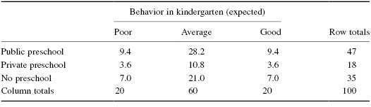
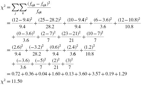
Using the values for the observed and expected frequencies in Tables 8.11 and 8.12, the χ2 statistic can be calculated:
8.4.2.5 Determine the Value Needed for Rejection of the Null Hypothesis Using the Appropriate Table of Critical Values for the Particular Statistic
Before we go to the table of critical values, we need to determine the degrees of freedom, df. In this example, there are three categories in the preschool experience dimension, R = 3, and three categories in the behavior dimension, C = 3. To find the degrees of freedom, use df = (R − 1)(C − 1) = (3 − 1)(3 − 1). Therefore, df = 4.
Now, we use Table B.2 in Appendix B, which lists the critical values for the χ2. The critical value is found in the χ2 table for four degrees of freedom, df = 4. Since we set α = 0.05, the critical value is 9.49. A calculated value that is greater than or equal to 9.49 will lead us to reject the null hypothesis.
8.4.2.6 Compare the Obtained Value with the Critical Value
The critical value for rejecting the null hypothesis is 9.49 and the obtained value is χ2 = 11.50. If the critical value is less than or equal to the obtained value, we must reject the null hypothesis. If instead, the critical value exceeds the obtained value, we do not reject the null hypothesis. Since the critical value is less than our obtained value, we must reject the null hypothesis.
8.4.2.7 Interpret the Results
We rejected the null hypothesis, suggesting that there is a real association between type of preschool experience children obtained and their behavior in the kindergarten classroom during their first few weeks in school. In particular, data tend to show that children who have private schooling do not tend to get good behavior ratings in school. The other area that tends to show some significant association is between poor behavior and no preschool experience. The students who had no preschool had very few poor behavior ratings in comparison with the other two groups.
At this point, the analysis is limited to identifying an association's presence or absence. In other words, the χ2-test's level of significance does not describe the strength of its association. The American Psychological Association (2001), however, has called for a measure of the degree of association called the effect size. For the χ2-test for independence with a 3 × 3 contingency table, we determine the strength of association, or the effect size, using Cramer's V.
From Table 8.11, we find that L = 3. For n = 100 and χ2 = 11.50, we use Formula 8.9 to determine V:
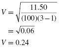
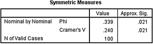
Our effect size, Cramer's V, is 0.24. This value indicates a medium level of association between type of preschool experience children obtained and their behavior in the kindergarten classroom during their first few weeks in school.
8.4.2.8 Reporting the Results
The reporting of results for the χ2-test for independence should include such information as the total number of participants in the sample and the number of participants classified in each of the categories. In addition, include the χ2 statistic, degrees of freedom, and the p-value's relation to α. For this study, the number of children who were in each category (including preschool experience and behavior rating) should be presented in the two-dimensional table (see Table 8.10).
For this example, the records of 100 kindergarten students were examined to determine whether there was an association between preschool experience and behavior in kindergarten. The three preschool experiences were no preschool, private preschool, and public preschool. The three behavior ratings were poor, average, and good. The χ2-test was significant (![]() , p < 0.05). Moreover, our effect size, using Cramer's V, was 0.24. Based on the results, there was a tendency shown for students with private preschool to not have good behavior and those with no preschool to not have poor behavior. It also indicated that average behavior was strong for all three preschool experiences.
, p < 0.05). Moreover, our effect size, using Cramer's V, was 0.24. Based on the results, there was a tendency shown for students with private preschool to not have good behavior and those with no preschool to not have poor behavior. It also indicated that average behavior was strong for all three preschool experiences.
8.4.3 Performing the χ2 Test for Independence Using SPSS
We will analyze the data from the example earlier using SPSS.
8.4.3.1 Define Your Variables
First, click the “Variable View” tab at the bottom of your screen, as shown in Figure 8.8. The χ2-test for independence requires variables to identify the conditions in the rows: one variable to identify the conditions of the rows and a second variable to identify the conditions of the columns. According to the previous example, the “Behavior” variable will represent the columns. “School_Type” will represent the rows. Finally, we need a variable to represent the observed frequencies. “Frequency” represents the observed frequencies.
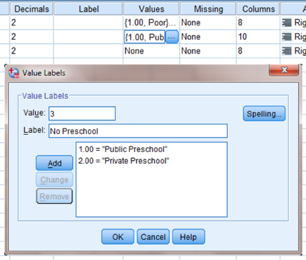
You must assign values to serve as a reference for the column and row variables. It is often easiest to assign each category a whole number value. First, click the gray square in the “Values” field to set the desired values. As shown in Figure 8.9, we have already assigned the value labels for the “Behavior” variable. For the “School_Type” variable, we set a value of 1 to equal “Public Preschool,” a value of 2 to equal “Private Preschool,” and a value of 3 to equal “No Preschool.” Clicking the “Add” button moves each of the value labels to the list below. Finally, click “OK” to return to the SPSS Variable View screen.
8.4.3.2 Type in Your Values
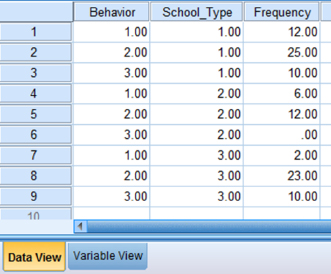
Click the “Data View” tab at the bottom of your screen, as shown in Figure 8.10. Use the whole number references you set earlier for the row and column variables. Each possible combination of conditions should exist. Then, enter the corresponding observed frequencies. In our example, row 1 represents a “Behavior” of 1 which is “Poor” and a “School_Type” of 1 which is “Public School.” The observed frequency for this condition is 12.
8.4.3.3 Analyze Your Data
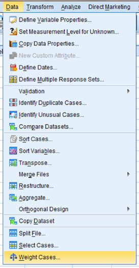
First, use the “Weight Cases” command to allow the observed frequency variable to reference the category variable. As shown in Figure 8.11, use the pull-down menus to choose “Data” and “Weight Cases …”.
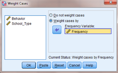
The default setting is “Do not weight cases.” Click the circle next to “Weight cases by” as shown in Figure 8.12. Select the variable with the observed frequencies. Move that variable to the “Frequency Variable:” box by clicking the small arrow button. In our example, we have moved the “Frequency” variable. Finally, click “OK.”
As shown in Figure 8.13, use the pull-down menus to choose “Analyze,” “Descriptive Statistics,” and “Crosstabs…”.
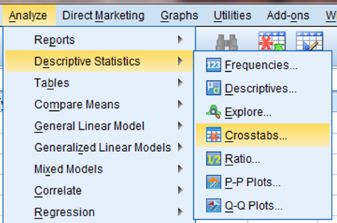
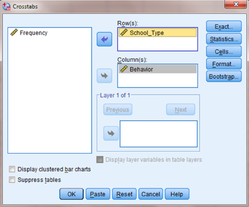
When the Crosstabs window is open, move the variable that represents the rows to the “Row(s):” box by selecting that variable and clicking the small arrow button next to that box. As shown in Figure 8.14, we have chosen the “School_Type” variable. Then, move the variable that represents the column to the “Column(s):” box. In our example, we have chosen the “Behavior” variable. Next, click the “Statistics …” button.
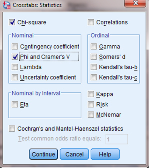
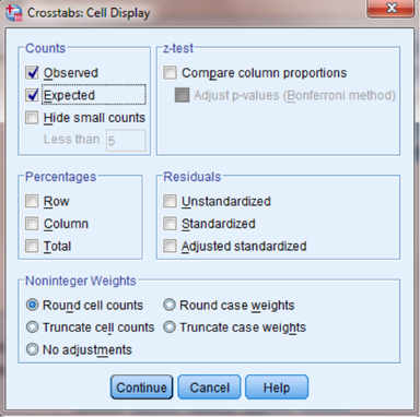
As shown in Figure 8.15, check the box next to “Chi-square” and the box next to “Phi and Cramer's V.” Once those boxes are checked, click “Continue” to return to the Crosstabs window. Now, click the “Cells …” button.
As shown in Figure 8.16, check the boxes next to “Observed” and “Expected.” Then, click “Continue” to return to the Crosstabs window. Finally, click “OK” to perform the analysis.
8.4.3.4 Interpret the Results from the SPSS Output Window
The second to fourth output tables from SPSS are of interest in this procedure. The second output table (see SPSS Output 8.2a) provides the observed and expected frequencies for each category and the total counts.
The third output table (see SPSS Output 8.2b) provides the χ2 statistic (χ2 = 11.502), the degrees of freedom (df = 4), and the significance (p = 0.021).
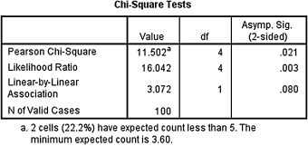
The fourth output table (see SPSS Output 8.2c) provides the Cramer's V statistic (V = 0.240) to determine the level of association or effect size.
Based on the results from SPSS, three programs were compared with unequal expected frequencies. The χ2 goodness-of-fit test was significant (![]() , p < 0.05). Based on these results, there is a real association between type of preschool experience children obtained and their behavior in the kindergarten classroom during their first few weeks in school. In addition, the measured effect size presented a medium level of association (V = 0.240).
, p < 0.05). Based on these results, there is a real association between type of preschool experience children obtained and their behavior in the kindergarten classroom during their first few weeks in school. In addition, the measured effect size presented a medium level of association (V = 0.240).
8.5 The Fisher Exact Test
A special case arises if a contingency table's size is 2 × 2 and at least one expected cell count is less than 5. In this circumstance, SPSS will calculate a Fisher exact test instead of a χ2-test for independence.
The Fisher exact test is useful for analyzing discrete data obtained from small, independent samples. They can be either nominal or ordinal. It is used when the scores of two independent random samples fall into one of two mutually exclusive classes or obtains one of two possible scores. The results form a 2 × 2 contingency table, as noted earlier.
In this chapter, we will describe how to perform and interpret the Fisher exact test for different samples.
8.5.1 Computing the Fisher Exact Test for 2 × 2 Tables
Compare the 2 × 2 contingency table's one-sided significance with the level of risk, α. Table 8.13 is the 2 × 2 contingency table that is used as the basis for computing Fisher exact test's one-sided significance.
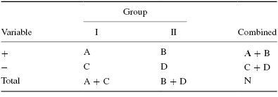
The formula for computing the one-sided significance for the Fisher exact test is shown in Formula 8.10. Table B.9 in Appendix B lists the factorials for n = 0 to n = 15:
If all cell counts are equal to or larger than 5 (ni ≥ 5), Daniel (1990) suggested that one use a large sample approximation with the χ2-test instead of the Fisher exact test.
8.5.2 Sample Fisher Exact Test
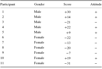
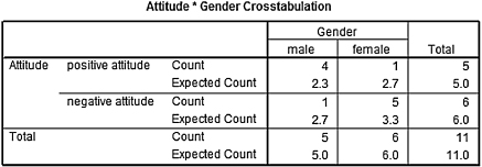
A small medical center administered a survey to determine its nurses' attitude of readiness to care for patients. The survey was a 15-item Likert scale with two points positive, two points negative, and a neutral point. The study was conducted to compare the feelings between men and women. Each person was classified according to a total attitude determined by summing the item values on the survey. A maximum positive attitude would be +33 and a maximum negative attitude would be −33.
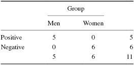
Table 8.14 and Table 8.15 show the number of men and women who had positive and negative attitudes about how they were prepared. There were four men and six women. Three of the men had positive survey results and only one of the women had a positive survey result.

We want to determine if there is a difference in attitude between men and women toward their preparation to care for patients. Since the data form a 2 × 2 contingency table and at least one cell has an expected count (see Formula 8.2) of less than 5, the Fisher exact test is a useful procedure to analyze the data and test the hypothesis.
8.5.2.1 State the Null and Research Hypotheses
The null hypothesis states that there are no differences between men and women on the attitude survey that measures feelings about the program that teaches care for patients. The alternative hypothesis is that the proportion of men with positive attitudes, PM, exceed the proportion of women with positive attitudes, PW.
The hypotheses can be written as follows.
HO: PM = PW
HA: PM > PW
8.5.2.2 Set the Level of Risk (or the Level of Significance) Associated with the Null Hypothesis
The level of risk, also called an alpha (α) level, is frequently set at 0.05. We will use α = 0.05 in our example. In other words, there is a 95% chance that any observed statistical difference will be real and not due to chance.
8.5.2.3 Choose the Appropriate Test Statistic
The data are obtained from a 2 × 2 contingency table. Two independent groups were measured on a survey and classified according to two criteria. The classifications were (+) for a positive attitude and (−) for negative attitude. The samples are small, thus requiring nonparametric statistics. We are analyzing data in a 2 × 2 contingency table and at least one cell has an expected count (see Formula 8.2) of less than 5. Therefore, we will use the Fisher exact test.
8.5.2.4 Compute the Test Statistic
First, construct the 2 × 2 contingency tables for the data in the study and for data that represent a more extreme occurrence than that which was obtained. In this example, there were five men and six women who were in the training program for nurses. Four of the men responded positively to the survey and only one of the women responded positively. The remainder of the people in the study responded negatively.
If we wish to test the null hypothesis statistically, we must consider the possibility of the occurrence of the more extreme outcome that is shown in Table 8.16b. In that table, none of the men responded negatively and none of the women responded positively.
To be shown later are the tables for the statistic. Table 8.16a show the results that occurred in the data collected and Table 8.16b shows the more extreme outcome that could occur.

To test the hypothesis, we first use Formula 8.10 to compute the probability of each possible outcome shown earlier.
For Table 8.16a,
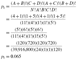
For Table 8.16b,
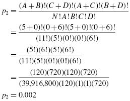
The probability is found by adding the two results that were computed earlier:
8.5.2.5 Determine the Value Needed for Rejection of the Null Hypothesis Using the Appropriate Table of Critical Values for the Particular Statistic
In the example in this chapter, the probability was computed and compared with the level of risk specified earlier, α = 0.05. This computational process involves very large numbers and is aided by the table values. It is recommended that a table of critical values be used when possible.
8.5.2.6 Compare the Obtained Value with the Critical Value
The critical value for rejecting the null hypothesis is α = 0.05 and the obtained p-value is p = 0.067. If the critical value is greater than the obtained value, we must reject the null hypothesis. If the critical value is less than the obtained value, we do not reject the null hypothesis. Since the critical value is less than the obtained value, we do not reject the null hypothesis.
8.5.2.7 Interpret the Results
We did not reject the null hypothesis, suggesting that no real difference existed between the attitudes of men and women about their readiness to care for patients. There was, however, a strong trend toward positive feelings on the part of the men and negative feelings on the part of the women. The probability was small, although not significant. This is the type of study that would call for further investigation with other samples to see if this trend was more pronounced. Our analysis does provide some evidence that there is some difference, and if analyzed with a more liberal critical value such as α = 0.10, this statistical test would show significance.
Since the Fisher exact test was not statistically significant (p > α), we may not have an interest in the strength of the association between the two variables. However, a researcher wishing to replicate the study may wish to know that strength of association.
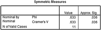
The effect size is a measure of association between two variables. For the Fisher exact test, which has a 2 × 2 contingency table, we determine the effect size using the phi (ϕ) coefficient (see Formula 8.8). For n = 11 and χ2 = 4.412 (calculation for χ2 not shown), we use Formula 8.8 to determine ϕ:

Our effect size, the phi (ϕ) coefficient, is 0.633. This value indicates a strong level of association between the two variables. What is more, a replication of the study may be worth the effort.
8.5.2.8 Reporting the Results
When reporting the findings, include the table that shows the actual reported frequencies, including all marginal frequencies. In addition, report the p-value and its relationship to the critical value.
For this example, Table 8.15 would be reported. The obtained significance, p = 0.067, was greater than the critical value, α = 0.05. Therefore, we did not reject the null hypothesis, suggesting that there was no difference between men and women on the attitude survey that measures feelings about the program that teaches care for patients.
8.5.3 Performing the Fisher Exact Test Using SPSS
As noted earlier, SPSS performs a Fisher exact test instead of a χ2-test for independence if the contingency table's size is 2 × 2 and at least one expected cell count is less than 5. In other words, to perform a Fisher exact test, use the same method you used for a χ2-test for independence.
SPSS Outputs 8.3a and 8.3b provide the SPSS output for the sample Fisher exact test computed earlier. Note that all four expected counts were less than 5. In addition, the one-sided significance is p = 0.067.
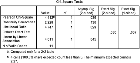
SPSS Output 8.3c provides the effect size for the association. Since the association was not statistically significant (p > α), the effect size (ϕ = 0.633) was not of interest to this study.
8.6 Examples from the Literature
Listed are varied examples of the nonparametric procedures described in this chapter. We have summarized each study's research problem and researchers' rationale(s) for choosing a nonparametric approach. We encourage you to obtain these studies if you are interested in their results.
Duffy and Sedlacek (2007) examined the surveys of 3570 1st-year college students regarding the factors they deemed most important to their long-term career choice. χ2 analyses were used to assess work value differences (social, extrinsic, prestige, and intrinsic) in gender, parental income, race, and educational aspirations. The researchers used χ2-tests for independence since these data were frequencies of nominal items.
Ferrari et al. (2006) studied the effects of leadership experience in an academic honor society on later employment and education. Drawing from honor society alumni, the researchers compared leaders with nonleaders on various aspects of their graduate education or employment. Since most data were frequencies of nominal items, the researchers used χ2-test for independence.
Helsen et al. (2006) analyzed the correctness of assistant referees' offside judgments during the final round of the FIFA 2002 World Cup. Specifically, they use digital video technology to examine situations involving the viewing angle and special position of a moving object. They used a χ2 goodness-of-fit test to determine if the ratio of correct to incorrect decisions and the total number of offside decisions were uniformly distributed throughout six 15-min intervals. They also used a χ2 goodness-of-fit test to determine if flag errors versus nonflag errors led to a judgment bias.
Shorten et al. (2005) analyzed a survey of 34 academic libraries in the United States and Canada that use the Dewey decimal classification (DDC). They wished to determine why these libraries continue using DDC and if they have considered reclassification. Some of the survey questions asked participants to respond to a reason by selecting “more important,” “less important,” or “not a reason at all.” Responses were analyzed with a χ2 goodness-of-fit test to examine responses for consensus among libraries.
Rimm-Kaufman and Zhang (2005) studied the communication between fathers of “at-risk” children with their preschool and kindergarten schools. Specifically, they examined frequency, characteristics, and predictors of communication based on family sociodemographic characteristics. When analyzing frequencies, they used χ2-tests. However, when cells contained frequencies of zero, they used a Fisher exact test.
Enander et al. (2007) investigated a newly employed inspection method for self-certification of environmental and health qualities in automotive refinishing facilities. They focused on occupational health and safety, air pollution control, hazardous waste management, and wastewater discharge. A Fisher exact test was used to analyze 2 × 2 tables with relatively small observed cell frequencies.
To examine the clinical problems of sexual abuse, Mansell et al. (1998) compared children with developmental disabilities to children without developmental disabilities. Categorical data were analyzed with χ2-tests of independence; however, the Yates' continuity corrections were used when cell counts exhibited less than the minimum expected count needed for the χ2-test.
8.7 Summary
Nominal, or categorical, data sometimes need analyses. In such cases, you may be seeking to determine if the data statistically match some known or expected set of frequencies. Or, you may wish to determine if two or more categories are statistically independent. In either case, nominal data can be analyzed with a nonparametric procedure.
In this chapter, we presented three procedures for examining nominal data: chi-square (χ2) goodness of fit, χ2-test for independence, and the Fisher exact test. We also explained how to perform the procedures using SPSS. Finally, we offered varied examples of these nonparametric statistics from the literature. In the next chapter, we will describe how to determine if a series of events occurred randomly.
8.8 Practice Questions
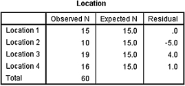
1. A police department wishes to compare the average number of monthly robberies at four locations in their town. Use equal categories in order to identify one or more concentrations of robberies. The data are presented in Table 8.17.
Use a χ2 goodness-of-fit test with α = 0.05 to determine if the robberies are concentrated in one or more of the locations. Report your findings.
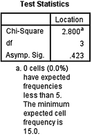
2. The χ2 goodness-of-fit test serves as a useful tool to ensure that statistical samples approximately match the desired stratification proportions of the population from which they are drawn.
A researcher wishes to determine if her randomly drawn sample matches the racial stratification of school age children. She used the most recent U.S. Census data, which was from 2001. The racial composition of her sample and the 2001 U.S. Census proportions are displayed in Table 8.18.
Use a χ2 goodness-of-fit test with α = 0.05 to determine if the researcher's sample matches the proportions reported by the U.S. Census. Report your findings.
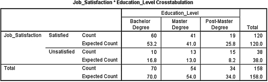
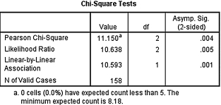
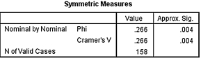
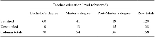
3. A researcher wishes to determine if there is an association between the level of a teacher's education and his/her job satisfaction. He surveyed 158 teachers. The frequencies of the corresponding results are displayed in Table 8.19.
First, use a χ2-test for independence with α = 0.05 to determine if there is an association between level of education and job satisfaction. Then, determine the effect size for the association. Report your findings.
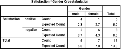
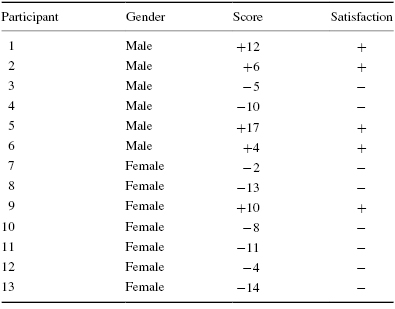
4. A professor gave her class a 10-item survey to determine the students' satisfaction with the course. Survey question responses were measured using a five-point Likert scale. The survey had a score range from +20 to −20. Table 8.20 shows the scores of the students in a class of 13 students who rated the professor.
Use a Fisher exact test with α = 0.05 to determine if there is an association between gender and course satisfaction of the professor's class. Then, determine the effect size for the association. Report your findings.
| Average monthly robberies | |
|---|---|
| Location 1 | 15 |
| Location 2 | 10 |
| Location 3 | 19 |
| Location 4 | 16 |
| Race | Frequency of race from the researcher's randomly drawn sample | Racial percentage of U.S. school children based on the 2001 U.S. Census (%) |
|---|---|---|
| White | 57 | 72 |
| Black | 21 | 20 |
| Asian, Hispanic, or Pacific Islander | 14 | 8 |
8.9 Solutions to Practice Questions
1. The results from the analysis are displayed in SPSS Outputs 8.4a and 8.4b.
According to the data, the results from the χ2 goodness-of-fit test were not significant (![]() , p > 0.05). Therefore, no particular location displayed a significantly higher or lower number of robberies.
, p > 0.05). Therefore, no particular location displayed a significantly higher or lower number of robberies.
2. The results from the analysis are displayed in SPSS Outputs 8.5a and 8.5b.
According to the data, the results from the χ2 goodness-of-fit test were significant (![]() , p < 0.05). Therefore, the sample's racial stratification approximately matches the U.S. Census racial composition of school aged children in 2001.
, p < 0.05). Therefore, the sample's racial stratification approximately matches the U.S. Census racial composition of school aged children in 2001.
3. The results from the analysis are displayed in SPSS Outputs 8.6a–8.6c.
As seen in SPSS Output 8.6a, none of the cells had an expected count of less than 5. Therefore, the χ2-test was indeed an appropriate analysis. Concerning effect size, the size of the contingency table was larger than 2 × 2. Therefore, a Cramer's V was appropriate.
According to the data, the results from the χ2-test for independence were significant (![]() , p < 0.05). Therefore, the analysis provides evidence that teacher education level differentiates between individuals based on job satisfaction. In addition, the effect size (V = 0.266) indicated a medium level of association between the variables.
, p < 0.05). Therefore, the analysis provides evidence that teacher education level differentiates between individuals based on job satisfaction. In addition, the effect size (V = 0.266) indicated a medium level of association between the variables.
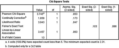
4. The results from the analysis are displayed in SPSS Outputs 8.7a–8.7c.
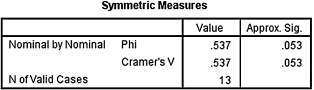
As seen in SPSS Output 8.7a, all of the cells had an expected count of less than 5. Therefore, the Fisher exact test was an appropriate analysis. Concerning effect size, the size of the contingency table was 2 × 2. Therefore, a phi (ϕ) coefficient was appropriate.
According to the data, the results from the Fisher exact test were not significant (p = 0.086) based on α = 0.05. Therefore, the analysis provides evidence that no association exists between gender and course satisfaction of the professor's class. In addition, the effect size (ϕ = 0.537) was not of interest to this study due to the lack of significant association between variables.