CHAPTER

9

Big Data, Business Intelligence, and Data Warehousing New Features

Oracle Database has always had features to help you scale your database size for almost any application, whether it be for OLTP or data warehouse applications. The key database feature for scaling both of those application types is table and index partitioning: the less data you have to sift through to get the results you want, the better your response time will be when you run queries or run your nightly ETL. In the first part of this chapter, I’ll cover a few of the new partitioning features in Oracle Database 12c Release 2, including enhancements to list partitioning and partitioning external tables.

In the last part of the chapter, I’ll describe a key enhancement to materialized views: real-time materialized view refresh. I’ll demonstrate how that feature can minimize the frequency of full materialized refreshes as well as meet the SLA with your user community to ensure consistent (and fast) query execution times when leveraging materialized views.

Leveraging New Partitioning Methods

Leveraging Oracle partitioning is the key to scaling any “big data” or data warehouse application that approaches the terabyte size. Partitioning is even beneficial for large OLTP applications that need to retrieve more a than few rows for a specific date range while e-commerce applications are servicing customer-facing web page and shopping cart checkout requests.

To recap the architecture and types of Oracle partitioning available for tables and indexes, here are the five you’ll have available to you in your partitioning toolbox:

   Range Each partition contains rows for a specific numeric or date range, most often a date range (year, month, week, day, even minutes if you want!).

   Hash Rows are spread out based on a hashing algorithm of the partitioning key to N different partitions, with each partition containing about the same number of rows.

   List Values of the partitioning key are explicitly mapped to a specific partition.

   System Partition mapping is determined within the application.

   External Partitions are stored as files on an OS file system, in Apache Hive storage, or on a Hadoop Distributed File System (HDFS).

Figure 9-1 shows typical examples of how you’d use list, range, and hash partitioning. In this chapter, I’ll describe the features and benefits of external table partitioning, new to Oracle Database 12c Release 2.

FIGURE 9-1. Examples of list, range, and hash partitioning

Furthermore, you can extend partitioning to a second level. In other words, you can use one primary partitioning method and, within each of those partitions, use another partitioning method to logically divide each primary partition. Secondary partitioning is also known as composite partitioning. All nine combinations of range, hash, and list partitioning are supported for composite partitioning: for example, range-hash, hash-range, list-list, and so forth.

There are many extensions to partitioning:

   Interval partitioning Creates a new range-based partition automatically when a new row doesn’t currently have an existing partition

   Interval subpartitioning Uses interval partitioning at the first level of a composite-partitioned table

   Reference partitioning Partitions a child table based on the foreign key column referencing the parent table with a foreign key constraint

   Multicolumn list partitioning An extension to list partitioning that uses more than one column to map a row to a partition based on each combination of values in those columns

   Automatic list partitioning Creates new partitions for a list partition when all values for the partition key are not known or new values will appear in the future

   Virtual column-based partitioning Uses an expression based on table columns instead of a physical column to calculate destination partition

Of the extensions listed above, interval subpartitions, multicolumn list partitions, and automatic list partitions are new to Oracle Database 12c Release 2 and are covered in the following sections. For example, when using range partitioning, you can further refine it by using interval partitioning to automatically create new partitions (which keeps rows out of your “catch-all” partition often called PMAX!). The biggest restriction on interval partitioning in general is that the column used for calculating the interval must not be NULL—otherwise, Oracle has no way to know which partition to put the new row into.

Using Interval Partitioning with Subpartitions

Interval partitioning was one of the most useful new features introduced in Oracle Database 11g Release 1 to enhance scalability and ease of maintenance for range-partitioned tables. If you have a partitioned table whose partition key is a date column (or a numeric column with values generated by a sequence), you have to stay ahead of the current possible values for the partitioning key—for example, your ORDERS table is likely partitioned by ORDER_DATE. If you want to make sure all new orders don’t end up in the partition defined by MAXVALUE, you have to stay at least one interval ahead of today’s date. In other words, if today is April 30, 2017, you want to make sure that a new partition is available for May 1, 2017, before the first order is placed after midnight on May 1.

Oracle Database 11g Release 1 solved this issue by allowing you to create range-partitioned tables with the INTERVAL clause, as in this example:

Your interval can be any unit of time or numeric value as long as you don’t exceed the 1 million partition limit for a partitioned table.

In Oracle Database 12c Release 2, you can use interval partitioning as the first level of a composite-partitioned table, with the second level being range, hash, or list partitioned. Here’s an example I created with composite range-list partitioning and the range partition using interval partitioning:

There are a few things to note in this example. This ORDERS table is range partitioned by day—every day’s set of orders has its own partition, but if there were any orders before January 1, 2001, they will end up in partition P0 with system-generated partitions for every day starting on January 1, 2001 if there is a row inserted for a given day.

Within each daily partition, there can be up to four subpartitions called EASTCOAST, WESTCOAST, MIDWESTCOAST, and OTHERCOAST. Rows that have a state code of WI will end up in the MIDWESTCOAST subpartition, rows with a state code of CA will end up in the WESTCOAST subpartition, and so forth. Any state codes not explicitly declared in the subpartition template will end up in the OTHERCOAST subpartition.

To find out what the partition structure looks like for the ORDERS table after a few days of orders from around the country, I ran a couple of queries like this:

New orders over the last few days have created three new range partitions on ORDER_DT. Digging deeper into the subpartitions, I ran this query:

Each of the partitions in the previous query has four subpartitions whether they have rows inserted or not; if you create those partitions with the clause SEGMENT CREATION DEFERRED, they won’t occupy any space other than as a row in the data dictionary.

List Partitioning Enhancements

Distinct values for a partitioned table help your performance and scalability in this way: referencing a partitioning column in a WHERE clause will perform partition pruning much like any other partitioning method—fewer partitions need to be considered for returning results to the query, which means less I/O and less elapsed time. However, with list partitioning in Oracle Database 12c Release 1 and earlier, you have to declare a DEFAULT partition for list-partitioned tables so that any partition key that is not part of any partition’s VALUE clause maps to the DEFAULT partition instead of generating an error. However, the DEFAULT partition may end up having quite a few values that might make that partition much larger than the other partitions—as a result, performance for queries referencing rows in the DEFAULT partition will likely suffer.

In the next two sections, I’ll describe two enhancements to list partitioning to enhance both scalability and manageability: automatic list partitioning and multicolumn list partitioning.

Automatic List Partitioning

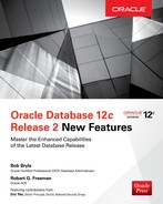
List partitioning has been available for several previous versions of Oracle Database, and its first incarnation let you specify one or more partition key values that map to one or more partitions, as in this example:

That worked fine when you did an INSERT like this:

But this was a problem:

To solve this issue in Oracle Database 12c Release 1 and earlier, you had to create the table like this instead:

The second INSERT would then work fine:

There was still a problem: unless you constantly monitored for customers in states that never ordered before, all other customer rows outside of the states defined in EASTCOAST, WESTCOAST, and MIDWESTCOAST ended up in OTHERCOAST, potentially making the OTHERCOAST partition so big that the benefits of partitioning were diminished when looking for a row in OTHERCOAST. Oracle Database 12c Release 2 addresses this issue by allowing automatic list partitioning.

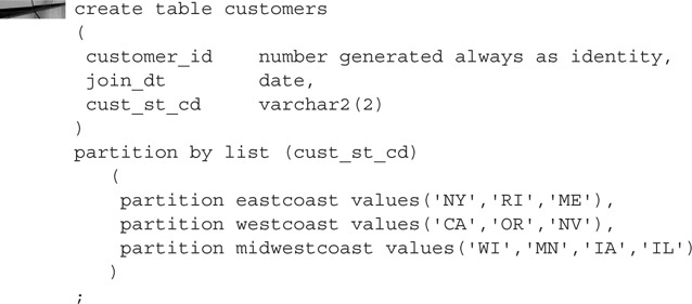
Automatic list partitioning is much like interval partitioning (reviewed extensively at the beginning of the chapter) except that you can use new discrete column values (numeric or character strings) to automatically create a new partition or subpartition to hold the new row. Modifying the structure of the CUSTOMERS table one more time, I use the AUTOMATIC keyword so that I don’t have to worry about creating new partitions manually when new values suddenly show up in the daily INSERT statements:

Using the AUTOMATIC keyword is not compatible with the DEFAULT list partitioning method, and that makes sense because you no longer need a DEFAULT partition if new partitions are automatically created every time a row with a new value for the partition key is inserted into the table. When I perform a number of inserts like this:

I can query DBA_TAB_PARTITIONS and see that a new partition was automatically created for the INSERT statement with ST_CD='AZ' since there was no existing partition that had AZ in its value list:

No new partitions were created for rows containing a state code of WI, MN, and IL since those partitions already existed right after the table was created.

Multicolumn List Partitioning

In Oracle Database 12c Release 1, you can create multicolumn range-partitioned tables with up to 16 columns in the PARTITION BY RANGE clause. For example, if you have separate numeric columns in your table for year and month instead of a single column with a DATE datatype, you can create a range-partitioned table using the YEAR and MONTH columns like this:

What if you want to have a multicolumn list-partitioned table? That’s not possible in Oracle Database 12c Release 1, but it is in Oracle Database 12c Release 2! For example, I just added the column CUST_TYP_CD to my CUSTOMERS table, and I want to further subdivide a given state’s customers by CUST_TYP_CD. However, because of how small the Wisconsin customer base is overall, I want all customer types in the same partition. I’m in luck, because in Oracle Database 12c Release 2, I can create a table with multicolumn list partitioning. Here’s the latest version of the CUSTOMERS table:

All business customers from New York will be stored in the EASTCOAST_BUS partition and all retail consumers from California will end up in the WESTCOAST_CON partition. All customers from Wisconsin, regardless of their customer type, will be stored in the MIDWESTCOAST partition. Any other combinations of state code and customer type will end up in the OTHER_COASTS partition—I specify that mapping by using the familiar VALUES(DEFAULT) clause.

You can have up to 16 columns in a multicolumn list-partitioned table. In this example, I have four identifiers in each table row and I want certain combinations to end up in specific partitions:

This can get quite complicated very quickly—not necessarily from a performance perspective but from a partition management perspective. However, it could be useful in cases where you want to more precisely control partition placement and therefore have more control over query performance.

Partitioning External Tables

The capability to partition external tables in Oracle Database 12c Release 2 is a natural extension to partitioning internal tables and has many of the advantages such as partition pruning and partition-wise joins. Partitioned external tables have similar restrictions to nonpartitioned external tables that you are already familiar with, such as being read-only and not supporting indexes. In the following sections, I’ll show you how to create and use partitioned external tables and also tell you what to watch out for.

New Access Drivers for Partitioned External Tables

As of Oracle Database 12c Release 1, the only two access drivers for external tables were ORACLE_LOADER and ORACLE_DATAPUMP. The ORACLE_LOADER driver looks much like a control file for the SQL*Loader utility, and that’s no accident—the ORACLE_LOADER driver enables you to create an external table that lets you access an OS flat file as if it were a native database table using syntax from a SQL*Loader control file. The other driver, ORACLE_DATAPUMP, enables you to write table data to an OS file and load it back into another Oracle database using the same driver.

In Oracle Database 12c Release 2, the ORACLE_HIVE driver enables you to access Apache Hive data as if it were a native database table; similarly, the ORACLE_HDFS access driver can map data in a Hadoop Distributed File System (HDFS) to database tables. To demonstrate how partitioned external tables work, I’ll use the ORACLE_LOADER driver because an in-depth discussion of Apache Hive and HDFS is beyond the scope of this book.

Creating Partitioned External Tables

Creating a partitioned external table is not much different from creating an external table in previous releases of Oracle Database, and most of the partitioning options available for native Oracle tables are available for external tables. Before you can access the data in an external table, you need to perform these four steps:

1.   Establish one or more directories on the OS file system that are accessible to the oracle OS user.

2.   Create flat files in the OS file system directories containing the data to be mapped to external table partitions.

3.   Create one or more Oracle directory objects that point to the OS directories containing the external table data.

4.   Create the external table referencing the structure of the flat file and the Oracle directory objects that point to the OS file system.

Create OS File System Directory Locations There is nothing special about the OS file location where your external table data is located other than that it needs to be accessible by the oracle OS user. In this example, I’m creating the subdirectory exttab under /u01/app/oracle to hold my external table partitions:

Since I’m creating an external partitioned table, I might have several or hundreds of flat files and they don’t all need to be in the same directory. In fact, even if your external table is not partitioned, you can logically coalesce any number of flat files in several different directories and access them all through a single external table.

Populate the OS File System Here is the test data I’ll use to demonstrate partitioned external tables. It consists of three csv files: one for Wisconsin, one for California, and a third for all other states.

The traditional partitioned table that would hold this data would look like this:

All three of these files are stored in /u01/app/oracle/exttab on my server:

Create Oracle Directory Objects Creating the directory object to reference the external table partitions is the same as in previous releases:

Create the Partitioned External Table Finally, I get to the good part: creating the table itself. It looks much like creating an external table in previous releases but with the addition of the PARTITION BY clause:

The new part of this CREATE TABLE statement is the PARTITION BY LIST clause where I specify not only the partition values but also the flat file location in the directory where those rows are stored.

Querying the Partitioned External Table Running a couple of queries on the CUSTOMERS_EXT table looks like running queries on a table stored natively in the database, and you wouldn’t suspect otherwise if the name of the table didn’t have EXT in it!

One of the best reasons to use partitioned external tables is to leverage partition pruning and as a result reduce the number of external files you need to scan every time you access the CUSTOMERS_EXT table. But how do you know that partition pruning is happening in the second SELECT statement? Check the execution plan! Figure 9-2 shows the output from an EXPLAIN PLAN in Oracle SQL Developer.

FIGURE 9-2. EXPLAIN PLAN on the CUSTOMERS_EXT query

The columns PARTITION_START and PARTITION_STOP in Figure 9-2 confirm that the query will only be accessing one partition (and therefore only one external table), which in this case is the external table with the rows from California.

Restrictions on Partitioned External Tables

There are a few restrictions on partitioned external tables besides the restrictions you would expect on nonpartitioned external tables, such as not being able to create indexes on external tables. Here are the most important restrictions:

   There is no validation that the rows in the external partition satisfy the definition of the VALUES clause for that partition.

   You cannot perform MODIFY PARTITION, EXCHANGE PARTITION, MERGE PARTITIONS, SPLIT PARTITION, COALESCE PARTITION, or TRUNCATE PARTITION operations on a partitioned external table.

   Reference, automatic list, and interval partitioning are not supported.

   Incremental statistics are not collected for partitions of a partitioned external table.

The first restriction is the one you need to carefully consider when evaluating partitioned external tables: your partition for CA could have non-CA rows in it and the query processing would not validate the partitioning key because it only accesses the corresponding external CSV file when the partition key in the WHERE clause matches the value in the VALUES clause. Adding a line in cust_ca.csv that has a state code of IL produces unexpected results:

Therefore, when using partitioned external tables, you’ll have to perform additional validations to ensure that the partitioning key column matches the value of the partition key as defined in the corresponding VALUES clause.

Materialized View Performance Improvements

Materialized views, available since Oracle Database 10g, provide huge scalability benefits in terms of reduced execution time at the expense of additional disk space. For example, if you have users in several departments who will aggregate employee or sales data several times a day, you can use materialized views to pre-aggregate the results of a query that has a GROUP BY clause. Even if a typical query only accesses a subset of departments or customer orders, the materialized view rewrite feature, enabled with the ENABLE QUERY REWRITE clause, will still use the aggregated query results in the materialized view and only return the rows relevant to the subset of departments.

The problem you often run into with materialized views is unexpected degradation in elapsed time when a materialized view becomes stale. For example, let’s say that after the nightly ETL you build an aggregated materialized view that sums daily order total by customer. It takes about 15 minutes to build the materialized view and each department’s query during the day only takes a few seconds to run since the order totals have already been computed for yesterday’s sales.

However, let’s say there was a duplicate item on one customer order and the duplicate item was deleted from the ORDER_ITEMS table—the materialized view you create every morning has now become stale and won’t be used for query rewrite for the rest of the day. You could potentially refresh the materialized view every time a change is made during the day to the ORDERS and ORDER_ITEMS table, but that takes 15 minutes and the impact on overall system performance will be high.

To address this problem (and prevent users from calling you when their reports suddenly take too long to run), Oracle Database 12c Release 2 now supports real-time materialized views. A real-time materialized view will still use a stale materialized view to support a query against the base tables and temporarily apply any changes to the base tables on the fly. To use this feature, you add the ENABLE ON QUERY COMPUTATION clause to your CREATE MATERIALIZED VIEW command, as in this example:

There are two new clauses you need to specify if you want to use real-time materialized views:

   INCLUDING NEW VALUES When you create the materialized view logs to support the refresh of your materialized view, you need to specify the INCLUDING NEW VALUES clause so that any new rows in the base tables are marked to make it more efficient for the real-time materialized view refresh to occur.

   ENABLE ON QUERY COMPUTATION In the CREATE MATERIALIZED VIEW command itself, you add the clause ENABLE ON QUERY COMPUTATION so that a stale materialized view will not prevent a user query from leveraging the materialized view if only a few rows in the base table have been updated, inserted, or deleted.

Whether or not you use real-time materialized views depends on the size of the materialized view and the typical number of changes made to the base tables during the day but before the next full refresh. If the materialized view is millions of rows and only one or two rows in the ORDERS table have changed, the slight additional work needed to merge the contents of the existing materialized view with the latest changes is minor compared to using the base tables instead of the materialized view to satisfy the query.

Summary

The enhancements to partitioning in Oracle Database 12c Release 2 revolve around additional list partitioning features. The new automatic list partitioning feature saves you time when a new partition is created for a partition key value that you didn’t expect—meaning that the new key value will have its own partition instead of ending up in a default partition. The multicolumn list partitions feature means you’ll have even more granular control over which rows end up in which partition based on more than just one column. External tables have also been enhanced to allow for list partitioning, meaning that you can save disk space by leaving more types of data outside of your database (Hadoop and Apache Hive data, for example) as well as save I/O by leveraging partition pruning.

Materialized views have also been fine-tuned to be more granular—it’s no longer “all or nothing” when attempting to leverage query rewrite against a materialized view when it becomes stale due to DML on the base tables. Real-time materialized views will take a stale materialized view and apply recent base table changes on the fly for the duration of a query. This will reduce the need for more frequent materialized view refreshes as well as keep user queries from experiencing wide variations in run times due to stale materialized views.

In the next chapter, I’m going to switch gears a bit from big data and analytics features to the Oracle security and utility realm by introducing an enhanced security analysis tool along with significant improvements to Oracle Data Pump.