What Is the SQL Explain Plan?

The explain plan illustrates the execution plan for any SQL statement. It shows the tables and indexes Oracle will use when processing an SQL statement, as well as the order in which the tables and indexes will be used. The execution plan is the order of events that Oracle will follow to access data and process the SQL statement. The explain plan and execution plan are determined when SQL is presented to Oracle for execution. If an SQL statement's actual code does not change and the SQL statement is still in the library cache, Oracle will simply reuse the original execution plan.

Oracle9i enables you to store and reuse this execution plan, which is known as stored outlines, this feature was introduced in Oracle8i. If you develop and tune a SQL statement in a test environment to use a very specific execution plan in the production environment, stored outlines enable you to guarantee that a particular SQL statement used a certain execution plan.

The Oracle Optimizers

Oracle9i supports two optimizers, a rule-based optimizer and a cost-based optimizer. The optimizer determines which explain plan is best for any SQL statement. It is possible that the same explain plan will be generated differently with subsequent submissions of an SQL statement not previously found in the library cache. The stored outlines come in handy, therefore, if the same execution plan is desired.

The rule-based optimizer is the original Oracle optimizer and makes decisions based on how the SQL statement is physically coded and the existence of indexes. The cost-based optimizer, on the other hand, was introduced with Oracle6 and makes its decisions based on statistics gathered by the ANALYZE command.

The Rule-Based Optimizer

The rule-based optimizer uses 19 rules to determine the execution path for a SQL statement (see Listing 14.1). The lower the rank (the rules are ranked from 1–19, with 1 being the best), the better the SQL statement should perform. Changing the execution plan (tuning) is accomplished by forcing the rule-based optimizer to make different selections. For example, adding an index to a column in the WHERE clause would alter the rank. If you don't want to use an index, you can add a function to an indexed field in a WHERE clause, which changes the rank and effectively disables the use of the index for this particular SQL statement. How the SQL statement is physically coded, particularly the order of the tables listed in the FROM clause, has a dramatic effect on the rule-based optimizer.

For example, consider the concept of a driving table, or the table that is compared to the others in a join SQL statement (multiple tables listed in the FROM clause). Because Oracle parses SQL statements from back to front, the driving table in a rule-based optimized SQL statement is the last one listed in the SQL statement. A few other dependencies can affect this decision, but for the most part, substantial performance gains can be gotten just by changing the order of the tables in the FROM clause.

Listing 14.1. Rule-Based Optimizer Rules

Rank    Where Clause Rule
1       ROWID = constant
2       unique indexed column = constant
3       entire unique concatenated index = constant
4       entire cluster key = cluster key of object in same cluster
5       entire cluster key = constant
6       entire nonunique concatenated index = constant
7       nonunique index = constant
8       entire noncompressed concatenated index >= constant
9       entire compressed concatenated index >= constant
10      partial but leading columns of noncompressed concatenated index
11      partial but leading columns of compressed concatenated index
12      unique indexed column using the SQL statement BETWEEN or LIKE options
13      nonunique indexed column using the SQL statement BETWEEN or LIKE options
14      unique indexed column < or > constant
15      nonunique indexed column < or > constant
16      sort/merge
17      MAX or MIN SQL statement functions on indexed column
18      ORDER BY entire index
19      full table scans

The Cost-Based Optimizer

The cost-based optimizer makes its decisions based on a cost factor derived from statistics for the objects in the SQL statement. The ANALYZE SQL statement is used to collect these statistics. Oracle9i introduces a new method of collecting statistics. The DBMS_STATS package has quite a bit more power over the existing ANALYZE command, particularly when it comes to large objects and the need to estimate the number of rows to gather statistics. DBMS_STATS is able to do a sampling of data across the object, when the object is large. This is much better than the ESTIMATED rows of the ANALYZE command where the ANALYZE command simply used the first percentage of rows in the object. The cost-based optimizer bases its execution-path decisions strictly on these collected statistics, so it is important to keep the statistics fresh, particularly with objects that have many DML-type SQL statements.

You can enable the cost-based optimizer by collecting statistics. The INIT.ORA parameter OPTIMIZER_MODE must be set to CHOOSE or COST or FIRST_ROWS_n, or it can be set at the user-session level with the ALTER SESSION command. You can disable the cost-based optimizer easily by either resetting the INIT.ORA parameter OPTOMIZER_MODE or deleting the statistics. If the shared pool has any current SQL statements that have execution plans based on newer statistics, Oracle will invalidate the SQL in the shared pool, allowing it to be re-prepared using the new statistics the next time the SQL statement is executed.

Oracle9i has several new cost-based statistics considerations it can use. Like prior versions of Oracle, Oracle9i will use statistics gathered on particular objects. Along with these statistics, Oracle9i is also able to collect, save, and reset system statistics, information that is important to the cost-based optimizer to help it make better decisions.

Object level statistics are now gathered with the DBMS_STATS package GATHER_SCHEMA_STATS. This functionally replaces the ANALYZE command with the improvement that it gathers statistics for all the objects owned by a particular schema. This new method has the ability to auto sample the data across the object, based on the size of the object and the workspace available to Oracle9i. When using the cost-based optimizer, it makes its best decisions when all objects involved have statistics.

The GATHER_SCHEMA_STATS command has a couple of options when it comes to histograms. If the size option is set to SKEWONLY, then a histogram will be created no matter how the application is using the particular column. In the method_opt option, if the size option is set to AUTO, then the histogram will reflect how the application is using the particular column. It is recommended that when the first time statistics are gathered, that the SKEWONLY option is used and subsequent statistic gatherings should use the AUTO setting. It is also recommended that the option estimate_percent be set to DBMS_STATS.AUTOSAMPLE_SIZE (for example: estimate_percent => DBMS_ STATS.AUTOSAMPLE_SIZE).

System statistics are gathered and used using the DBMS_STATS package options: GATHER_SYSTEM_STATS, SET_SYSTEM_STATS, and GET_SYSTEM_STATS, and IMPORT_SYSTEM_STATS.

System statistics can differ greatly at different parts of the day and based on the types of applications being run at these various times of the day. GATHER_SYSTEM_STATS has a time element involved with it as well as the ability to give the collection a name. This name allows for different pre-collected statistics to be used at different times of the processing day. Listing 14.2 illustrates how this might be used on the first shift and second shift versus subsequent first and second shifts.

Listing 14.2. GATHER_SYSTEM_STATS Example

First Shift/First Day EXECUTE DBMS_STATS.GATHER_SYSTEM_STATS ( Interval => 90, Stattab => 'System A Stats', Statid => 'shift1'), Second Shift/First Day EXECUTE DBMS_STATS.GATHER_SYSTEM_STATS ( Interval => 90, Stattab => 'System A Stats', Statid => 'shift2'), First Shift/Next Day EXECUTE_DBMS_STATS.IMPORT_SYSTEM_STATS ( Stattab => 'System A Stats', Statid => 'shift1'), Second Shift/Next Day EXECUTE_DBMS_STATS.IMPORT_SYSTEM_STATS ( Stattab => 'System A Stats', Statid => 'shift2'),

SET_SYSTEM_STATS is used to explicitly set the system statistics and GET_SYSTEM_STATS is used to verify system statistics.

Hints are used to influence the cost-based optimizer and can be used to control the optimizer's goal, access methods, join conditions, parallel option, and partitioning option. Hints are specified in the SQL statement syntax. Listing 14.3 illustrates an ALL_ROWS hint in the SCOTT.EMP table.

Listing 14.3. Hints in SQL Statements

select /*+ ALL_ROWS */ ename, sal from EMP where SAL > 1000

Listing 14.4 shows most of the hints for controlling the execution plan available in Oracle9i. The cost-based optimizer also has the driving-table mechanism in join conditions. The ORDERED hint causes the driving table to be the first table in the FROM clause of the SQL statement.

Listing 14.4. Access Control Hints

Hint Description AND_EQUAL Use the AND_EQUAL hint when more than one equality criterion exists on a single table. CACHE Use the CACHE hint to place the entire table in the buffer cache. The table is placed at the most recently used end of the buffer cache. This hint is good for small tables that are accessed often. CLUSTER Use the CLUSTER hint to access a table in a cluster without the use of an index. FULL Use the FULL hint to perform a full table scan on a table. HASH Use the HASH hint to access a table in a hashed cluster without the use of an index. INDEX Use an INDEX hint to instruct ORACLE to use one of the indexes specified as a parameter. INDEX_COMBINE The INDEX_COMBINE forces the use of bitmap indexes. NOCACHE Use the NOCACHE hint to place the blocks of the table at the beginning of the buffer cache so as not to age any blocks out. NOPARALLEL Use the NOPARALLEL hint to not use multiple-server processes to service the operations on the specified table. ORDERED Use the ORDERED hint to access the tables in the FROM clause in the order they appear. PARALLEL Use the PARALLEL hint to request multiple server processes to simultaneously service the operations on the specified table. PUSH_SUBQ The PUSH_SUBQ evaluates subqueries earlier, rather than as a filter operation. ROWID Use the ROWID hint to access the table by ROWID. STAR STAR hint invokes the STAR query feature. USE_HASH Use the USE_HASH hint to perform a hash join rather than a merge join or a nested loop join. USE_MERE Use the USE_MERGE hint to perform a merge join rather than a nested loop join or a hash join.

Say you have a table full of names, with an index on the last name. Let's also say that this table has proportionately more occurrences of Jones and Smith than most of the other rows. A histogram would be useful in this example because data won't be evenly distributed throughout the table object. Prior to histograms, the Oracle optimizer assumed even distribution of values throughout the object.

Figure 14.1 illustrates a histogram as a series of buckets. Two kinds of histograms are available, width balanced and height balanced. Width-balanced histograms have values that are divided up into an even number of buckets, enabling the optimizer to easily determine which buckets have higher counts. In height-balanced histograms, however, each bucket has the same number of column values, but a column value can span more than one bucket. Figure 14.1 illustrates what the EMP table might look like in each of these types of histograms.

When two or more tables are joined together, Oracle must pull the columns from each table, creating a result set, which is a temporary table of sorts. This result set is created in the TEMPORARY tablespace and contains the combination of rows. The Oracle optimizer chooses one of five methods to perform this join: a nested-loop join, a sort-merge join, a hash join, a cluster join, and (new with Oracle8i) an index join. The most common joins are the first three listed here.

A nested-loop join reads the first row from the driving table, or outer table, and checks the other table, called the inner table, for the value. If the value is found then the rows are placed into the result set. Nested-loops work best when the driving table is rather small and a unique index is defined on the inner table's joined column.

A sort-merge join sorts both of the joined tables by the join column and then matches the output from these sorts. Any matches are subsequently placed into the result set. The big difference between this join and the nested-loop is that in the sort-merge, no rows are returned until after this matching process completes, whereas the nested-loop returns rows almost immediately. Nested-loops are a good choice when the first few rows need to be returned almost immediately. In contrast, sort-merge joins work better with larger amounts of data, or situations in which the two joining tables are roughly the same size and most of the rows will be returned. In practice, there seems to be no good reason to use a sort-merge join.

Hash joins can dramatically increase the performance of two joined tables in situations in which one table is significantly larger than the other. The hash join works by splitting two tables into partitions and creating a memory-based hash table. This hash table is then used to map join columns from the other table, eliminating the need for a sort-merge. In the hash join method, all tables are scanned only once. Hash joins are implemented by the INIT.ORA parameters HASH_JOIN_ENABLED, HASH_MULTIBLOCK_IO_COUNT, and HASH_AREA_SIZE. A star query involves a single table object being joined with several smaller table objects, where the driving table object has a concatenated index key and each of the smaller table objects is referenced by part of that concatenated key. The Oracle cost-based optimizer recognizes this arrangement and builds a memory-based cluster of the smaller tables.

Cluster joins are used instead of nested-loops when the join condition is making reference to tables that are physically clustered together. The Oracle cost-based optimizer recognizes this condition and uses the cluster join when the tables being joined are in the same cluster. Tables are candidates for clustering when they are joined together and no other queries are typically run against one or the other. Clustering physically aligns the joined column rows together in the same data block, which is why cluster joins are so efficient—the data is already being accessed with a single I/O to the database.

Index joins work on the concept that if all the information required for the SQL statement is found in the index, the underlying table structure is not accessed or referenced in the execution plan.

Figure 14.2 illustrates the differences in the times of the three main kinds of join conditions. Notice that the nested-loop starts out very fast, but the more rows processed, the slower it becomes. The sort-merge join starts off the slowest because it must sort and merge the columns before returning any rows; however, its overall performance is pretty consistent. The hash join, on the other hand, starts out quickly and has the overall best performance because all the columns in the join conditions have a hash key in the hash table, enabling very quick access to the data.

Which method is best? Once again, it depends on the application, the amount of data being joined, and so on.

Tuning SQL Statements

When we tune SQL statements at the application level, it is important that we are able to monitor and capture long-running, or very I/O-intensive, SQL statements. The old 80/20 rule generally applies here: 20% of the SQL statements are consuming 80% of the system resources. Being able to identify and tune the 20% is critical.

Oracle supplies a product called TKPROF, which is a character-mode tool used to interpret the contents of trace files. Trace files contain all the SQL statements and statistics for a particular trace session. Traces can be created by an INIT.ORA parameter or more importantly, by setting the trace function to on at the application level. For example, one of the options when starting an Oracle form is to trace the form. Traces also can be created by setting a session-level trace to on with a SQL statement, such as ALTER SESSION SET SQL_TRACE TRUE;.

The Oracle trace facility captures all the SQL statements, but TKPROF is not a tool for the novice, and finding specific poorly performing SQL statements might be difficult. Oracle also provides an explain plan facility, activated by running the script <ORACLE_HOME>/rdbms/admin/utlxplan.sql, for each user wanting to visualize explain plans (see Listing 14.5). A single explain plan table can be created and given public access, but if several people are performing SQL statement tuning, it is more convenient for them to simply create their own explain tables. Figure 14.3 illustrates using Quest Software SQLab Xpert to submit a SQL statement and the resulting explain plan. SQLab Xpert is very good at monitoring and finding poorly performing SQL statements across the system or for a particular session but also is an excellent SQL tuning environment. Notice that the resulting explain plans are very similar, but the SQLab, being a GUI environment, has many more features for actually tuning the SQL statement.

Listing 14.5. Oracle Explain Plan Using PLAN_TABLE

SQL> l 1 EXPLAIN PLAN INTO plan_table FOR 2 select sum(bt_time * staff_billing_rate) 3 from st_bill_time, st_staff 4 where st_bill_time.bt_inv_id = 14 5* and st_bill_time.bt_staff_id = st_staff.staff_id SQL> / Explained. SQL> SELECT cost, operation, options, object_name 2 FROM plan_table; COST OPERATION OPTIONS OBJECT_NAME --------- ------------------------------ ------------ ---------------------- 3 SELECT STATEMENT SORT AGGREGATE 3 HASH JOIN 1 TABLE ACCESS FULL ST_STAFF 1 TABLE ACCESS FULL ST_BILL_TIME

Understanding the explain plan is a necessity for tuning SQL statements for both the rule-based and cost-based optimizers. Explain plans can be difficult to interpret, but indenting the explain steps greatly aids in understanding the order of the explain steps. The more common explain steps are discussed in Listing 14.6.

Listing 14.6. Common Explain Plan Symbols

Explain Symbol                Description
AND-EQUAL                     Index values will be used to join rows.
CONCATENATION                 SQL statement UNION command.
FILTER                        FILTERs apply 'other criteria' in the query to
                              further qualify the matching rows. The 'other
                              criteria' include correlated subqueries, and
                              HAVING clause.
FIRST ROW                     SQL statement will be processed via a cursor.
FOR UPDATE                    SQL statement clause 'for update of' placed row
                              level locks on affected rows.
INDEX (UNIQUE)                SQL statement utilized a unique index to search
                              for a specific value.
INDEX (RANGE SCAN)            SQL statement contains a nonequality or BETWEEN
                              condition.
HASH JOIN                     SQL statement initiated a hash-join operation.
MERGE JOIN                    SQL statement references two or more tables,
                              sorting the two result sets being joined over the
                              join columns and then merging the results via
                              the join columns.
NESTED LOOPS                  This operation is one form of joining tables.
                              One row is retrieved from the row source
                              identified by the first (inner) operation, and
                              then joined to all matching rows in the other
                              table (outer).
NONUNIQUE INDEX (RANGE SCAN)  The RANGE SCAN option indicates that ORACLE
                              expects to return multiple matches (ROWIDs) from
                              the index search.
PARTITION (CONCATENATED)      SQL statement will access a partitioned object
                              and merge the retrieved rows from the accessed
                              partitions.
PARTITION (SINGLE)            SQL statement will access a single partition.
PARTITION (EMPTY)             The SQL statement makes reference to an empty
                              partition.
SORT (ORDER BY)               SQL statement contains an ORDER BY SQL command.
SORT (AGGREGATE)              SQL statement initiated a sort to resolve a MIN
                              or MAX function.
SORT (GROUP BY)               SQL statement contains a GROUP BY SQL command.
TABLE ACCESS (FULL)           All rows are retrieved from the table without
                              using an index.
TABLE ACCESS (BY ROWID)       A row is retrieved based on ROWID
TABLE ACCESS (CLUSTER)        A row is retrieved from a table that is part of
                              a cluster.
UNION                         SQL statement contains a DISTINCT SQL command.

Oracle version 8 has introduced three new columns: PARTITION_START, PARTITION_STOP, and PARTITION_ID. These three new fields will help in the tuning of SQL statements that access partitioned objects. PARTITION_START and PARTITION_STOP show the range of partitions affected by this explain step, and the PARTITION_ID is the identification number for that particular explain step.

The largest performance gains can be obtained by tuning the top four or five steps of the explain plan. Figure 14.4 illustrates one of the sales tracking SQL statements (from the Profit/Loss Calculation button in the ST_INVENTORY form). SQLab Xpert provides quite a bit of information—notice the indexes listed on the right side and all the column attributes listed as well. This particular SQL statement was captured via monitoring, which is discussed in Chapter 5, “Building Oracle Forms.” Notice that SQLab set up five scenarios using hints:

• Original SQL

• Rule Hint

• All_Rows Hint

• First_Rows Hint

• Ordered Hint

SQLab also has the capability to compare each of these scenarios.

In the SQL explain plan, SQLab indents and highlights each of the explain steps (see Figure 14.4). For the novice, SQLab also provides a meaningful explanation—in the box under the explain plan—of what each step really means. On the highlighted explain plan line, notice the Table Access Full, or a full table scan. Also notice the statistics, primarily the number of rows affected. Normally, a full table scan is a bad thing, but when only 21 rows are being affected, a full table scan is actually a good thing. Having an index would only increase the number of I/Os to retrieve this data, which is probably all in the same data block. In addition, notice the hash join in step 3 of the explain plan.

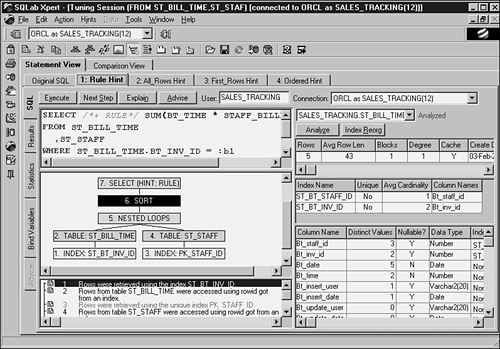
The example in Figure 14.5 is the same tuning session as in Figure 14.4, except the Rule Hint tab is the current tab. Using the rule-based optimizer, the optimizer picked a nested-loop join operation in step 5 of the explain plan because the rule-based optimizer does not support hash joins.

SQLab can actually give advice on how to rewrite the SQL statement. In Figure 14.6, the Advice tab on the left side of the screen shows that SQLab is recommending to drop the indexes. This recommendation comes because, in this case, the indexes will probably slow down the processing of this SQL statement due to the extra I/Os required to access the indexes. Notice that it is also advising either to analyze all the tables or to have none of them analyzed. Finally, this SQL statement recommends creating indexes on the foreign keys. The Generate SQL button will generate a SQL script to implement any of the recommendations selected.

The final SQLab example in Figure 14.7 illustrates another way of viewing the explain plan, in a flowchart mode. SQLab enables the user to toggle between the regular explain display mode and the flowchart mode, which provides a nice way to view the relationships in the explain plan.

The cost-based optimizer uses various statistics to make its decisions. One of the more important statistics is the concept of clustering factor.

Clustering factor is a relationship between the number of data blocks being referenced by each index leaf block. The better this relationship, that is, the fewer different data blocks referenced in each index leaf block, the better the clustering factor. This means for each read of the index leaf block, Oracle will have to do fewer data block reads to satisfy what is found in the index. This is very important when doing any kind of range-scan across the index. A lower clustering factor can be accomplished by sorting the table in the order of the main index that is to be used, prior to loading the table into Oracle.

Oracle9i can efficiently use concatenated key indexes where the WHERE clause does not contain the leading column of the concatenated key. Oracle9I has implemented a new index-search method called skip scanning. Skip scanning allows Oracle to scan the branch blocks looking for the non-leading key values and ignore the other index blocks.

There are four basic kinds of index scans that can be seen in the explain plan and set using a hint: unique index scan, range scan, full scan (shows up in the explain plan as INDEX_FULL), and fast full scan (shows up in the explain plan as INDEX_FSS).

A unique index scan probes the index tree structure for an individual row, using a unique index. The range scan probes the index tree structure for the first occurrence of the range, then reads leaf-to-leaf until the range is satisfied. A full scan scans leaf blocks using a single-block read and a fast full scan uses the multi-block read ahead method, skipping branch blocks and processing the leaf blocks.