
Parallel Property of Pressure Equation Solver with Variable Order Multigrid Method for Incompressible Turbulent Flow Simulations
Hidetoshi Nishidaa,*; Toshiyuki Miyanob a Department of Mechanical and System Engineering, Kyoto Institute of Technology, Matsugasaki, Sakyo-ku, Kyoto 606-8585, Japan
b Toyota Industries Corporation, Toyoda-cho 2-1, Kariya 448-8671, Japan
In this work, the parallel property of pressure equation solver with variable order multigrid method is presented. For improving the parallel efficiency, the restriction of processor elements (PEs) on coarser multigrid level is considered. The results show that the parallel property with restriction of PEs can be about 10% higher than one without restriction of PEs. The present approach is applied to the simulation of turbulent channel flow. By using the restriction of PEs on coarser multigrid level, the parallel efficiency can be improved in comparison with the usual without restriction of PEs.
1 INTRODUCTION
The incompressible flow simulations are usually based on the incompressible Navier-Stokes equations. In the incompressible Navier-Stokes equations, we have to solve not only momentum equations but also elliptic partial differential equation (PDE) for the pressure, stream function and so on. The elliptic PDE solvers consume the large part of total computational time, because we have to obtain the converged solution of this elliptic PDE at every time step. Then, for the incompressible flow simulations, especially the large-scale simulations, the efficient elliptic PDE solver is very important key technique.
In the parallel computations, the parallel performance of elliptic PDE solver is not usually high in comparison with the momentum equation solver. When the parallel efficiency of elliptic PDE solver is 90% on 2 processor elements (PE)s. that is. the speedup based on 1PE is 1.8. the speedup on 128PEs is about 61 times of 1PE. This shows that we use only the half of platform capability. On the other hand, the momentum equation solver shows almost theoretical speedup [1], [2]. Therefore, it is very urgent problem to improve the parallel efficiency of elliptic PDE solver.
In this paper, the parallel property of elliptic PDE solver, i.e., the pressure equation solver, with variable order multigrid method [3] is presented. Also, the improvement of parallel efficiency is proposed. The present elliptic PDE solver is applied to the direct numerical simulation (DXS) of 3D turbulent channel flows. The message passing interface (MPI) library is applied to make the computational codes. These MPI codes are implemented on PRIME POWER, system with SPARC 64V (1.3GHz) processors at Japan Atomic Energy Agency (JAEA).
2 NUMERICAL METHOD
The incompressible Navier-Stokes equations in the Cartesian coordinates can be written by

where ui (i = 1,2,3) denotes the velocity, p the pressure and v the kinematic viscosity. The pressure equation can be formally written by
where f is the source term.
2.1 Variable Order Method of Lines
The solution procedure of the incompressible Navier-Stokes equations (1) and (2) is based on the fractional step approach on the collocated grid system.
In the method of lines approach, the spatial derivatives arc discretized by the appropriate scheme, so that the partial differential equations (PDEs) in space and time are reduced to the system of ordinary differential equations (ODEs) in time. The resulting ODEs are integrated by the Runge-Kutta type time integration scheme.
In the spatial discretization, the convective terms are approximated by the variable order proper convective scheme [2], because of the consistency of the discrete continuity equation, the conservation property, and the variable order of spatial accuracy. This scheme is the extension of the proper convective scheme proposed by Morinishi [4] to the variable order. The variable order proper convective scheme can be described by

where M denotes the order of spatial accuracy, and the operators in eq.(4) are defined by

where m’ = 2m − 1. In this technique, the arbitrary order of spatial accuracy can be obtained automatically by changing only one parameter M. The coefficients cl′ and cm′ are the weighting coefficients and Δxj denotes the grid spacing in the xj direction.
On the other hand, the diffusion terms are discretized by the modified differential quadrature (MDQ) method [5] as

where φm″(x) is the second derivative of the function φm(x) defined by
The coefficients of the variable order proper convertive scheme, cℓ′ can be computed automatically by using the MDQ coefficients. Then, the incompressible Navier-Stokes equations are reduced to the system of ODEs in time. This system of ODEs is integrated by the Runge-Kutta type scheme.
2.2 Variable Order Multigrid Method
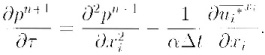
The pressure equation described by

is solved by the variable order multigrid method [3]. In eq.(11), ![]() denotes the fractional step velocity, α is the parameter determined by the time integration scheme. The overbar denotes the interpolation from the collocated location to the staggered location. In the variable order multigrid method, the unsteady term is added to the pressure equation. Then, the pressure (elliptic) equation is transformed to the parabolic equation in space and pseudo-time, τ.
denotes the fractional step velocity, α is the parameter determined by the time integration scheme. The overbar denotes the interpolation from the collocated location to the staggered location. In the variable order multigrid method, the unsteady term is added to the pressure equation. Then, the pressure (elliptic) equation is transformed to the parabolic equation in space and pseudo-time, τ.
Equation (12) can be solved by the variable order method of lines. The spatial derivatives are discretized by the aforementioned MDQ method, so that eq.(12) is reduced to the system of ODEs in pseudo-time.
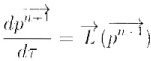
This system of ODEs in pseudo-time is integrated by the rational Runge-Kutta (RRK) scheme [6]. because of its wider stability region. The RRK scheme can be written by

where ∆τ and m are; the pseudo-time step and level, and the operators such as ![]() denote inner product of vectors
denote inner product of vectors ![]() and
and ![]() . Also the coefficients b1, b2, and c2 satisfy the relations b1 + b2 = 1, c2 = −1/2.
. Also the coefficients b1, b2, and c2 satisfy the relations b1 + b2 = 1, c2 = −1/2.
In addition, the multigrid technique [7] is incorporated into the method in order to accerelate the convergence. Then, the same order of spatial accuracy as the momentum equations can be specified.
3 MULTIGRID PROPERTY OF PRESSURE EQUATION SOLVER
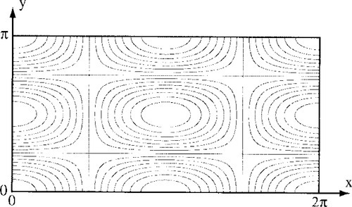
First, the 2D case with the source term f(x,y) = −5cos(x)cos(2y) and the Neumann boundary conditions ∂p/∂xi = 0 are considered. In order to compare the results, the point Jacobi (PJ) method and checkerboard SOR (CB-SOR) method arc considered as the relaxation scheme. Figure 1 shows the computational region and analytic solution.
3.1 Multigrid Property
Figure 2 shows the work unit until convergence. The comparison of computational time and work unit is shown in Table 1. The computation is executed with the second order of spatial accuracy. The present three relaxation schemes indicate the mulatigrid convergence. In these relaxation schemes, the RRK scheme gives the good multigrid property with respect to the work unit and computational time. In order to check the influence of spatial accuracy, the comparison of work unit is shown in Fig.3. In both relaxation schemes, the multigrid convergence; can be obtained and the RRK scheme has the independent property of spatial accuracy.

Table 1
Work unit and computational time.
| work | 256 × 128 | 512 × 256 | 1024 × 512 | 2048 × 1024 |
| P.J | 34.629 | 34.629 | 33.371 | 34.390 |
| CB-SOR | 22.655 | 22.666 | 22.666 | 23.917 |
| RRK | 17.143 | 15.583 | 16.833 | 16.000 |
| time (sec) | 256 × 128 | 512 × 256 | 1024 × 512 | 2048 × 1024 |
| PJ | 0.318 | 1.448 | 5.770 | 23.332 |
| CB-SOR | 0.238 | 0.847 | 3.650 | 15.218 |
| RRK | 0.255 | 0.943 | 1.405 | 16.448 |


3.2 Parallel Property
In order to implememt to a parallel platform, the domain decomposition technique; is used. In this work, 16 sub-domains are assigned to 16 PEs. Figure 4 shows the parallel efficiency defined by
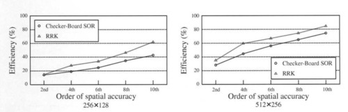
where N denotes number of PEs, Tsingle and Tparallel are the CPU time on single PE and N PEs, respectively. In both relaxation schemes, as the order of spatial accuracy becomes higher, the parallel efficiency becomes higher. The RRK scheme gives the higher efficiency than the checkerboard SOR method. In 2D multigrid method, from fine grid to coarse grid, the operation counts become 1/4, but the data transfer becomes 1/2. Then, the parallel efficiency on coarser grid will be lower, so that, the total parallel efficiency is not too high.
In order to improve parallel efficiency, we consider the restriction of PEs on coarser grid level. Figure 5 shows the parallel efficiency with the restriction of PEs on coarser than 64 × 32 grid level. In Fig.5, version 1 and version 2 denote the parallel efficiency without and with restriction of PEs on coarser grid level, respectively. It is clear that the parallel efficiency of version 2 can be about 10% higher than version 1.

4 TURBULENT CHANNEL FLOW SIMULATION
The DNS of 3D turbulent channel flows is performed by the variable order method of lines. The order of spatial accuracy is the 2nd order and the number of grid points are 32 × 64 × 32 and 64 × 64 × 64 in the x, y and z directions. The numerical results with Reynolds number Rcτ 150 are compared with the reference database of Kuroda and Kasagi [8] obtained by the spectral method. Figures 6 shows the mean streamwise velocity. Reynolds shear stress profiles, velocity fluctuation, and the iso-surface of second invariant of velocity gradient tensor, respectively. The present DNS results are in very good agreement with the reference spectral solution.
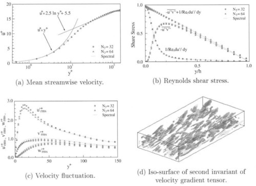
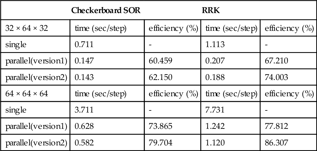
Table 2 shows the parallel efficiency of 2nd order multigrid method in the DNS of 3D turbulent channel flow. The parallelization is executed by the domain decomposition with 8 sub-domains. As the number of grid points becomes larger, the parallel efficiency becomes higher. The version 2 with restriction of PEs shows the higher parallel efficiency than the usual without restriction. In comparison with the checkerboard SOR method. the RRK scheme has the higher parallel efficiency not only in version 1 but also in version 2.
Table 2
Parallel efficiency for 3D turbulent channel flow.
| Checkerboard SOR | RRK | |||
| 32 × 64 × 32 | time (sec/step) | efficiency (%) | time (sec/step) | efficiency (%) |
| single | 0.711 | - | 1.113 | - |
| parallel(version1) | 0.147 | 60.459 | 0.207 | 67.210 |
| parallel(version2) | 0.143 | 62.150 | 0.188 | 74.003 |
| 64 × 64 × 64 | time (sec/step) | efficiency (%) | time (sec/step) | efficiency (%) |
| single | 3.711 | - | 7.731 | - |
| parallel(version1) | 0.628 | 73.865 | 1.242 | 77.812 |
| parallel(version2) | 0.582 | 79.704 | 1.120 | 86.307 |
5 CONCLUDING REMARKS
In this work, the parallel property of pressure equation solver with variable order multi-grid method is presented. For improving the parallel efficiency, the restriction of processor elements (PEs) on coarser multigrid level is considered. The results show that the parallel property with restriction of PEs can be about 10% higher than one without restriction of PEs. The present pressure equation solver is applied to the simulation of turbulent channel flow. The incompressible Navier-Stokes equations are solved by the variable order method of lines. By using the restriction of PEs on coarser multigrid level, the parallel efficiency can be improved in comparison with the usual without restriction of PEs. Therefore, the present approach is very hopeful for parallel computation of incompressible flows.
* This work was supported in part by a Grant-in-Aid for Scientific Research (16560146) from the Japan Society for the Promotion of Science. We would like to thank Japan Atomic Energy Agency (JAEA) for providing a parallel platform.