
Sensitivity study with global and high resolution meteorological model
Paola Mercoglianoa; Keiko Takahashib; Pier Luigi Vitaglianoa; Pietro Catalanoa a The Italian Aerospace Research Center (CIRA),Via Maio rise, 81043 Capua (CE), Italy
b Earth Simulator Centre (ESC), Japan Agency for Marine-Earth Science and Technology3173-25 Showa-machi, Kanazawa-ku, Yokohama Kanagawa 236-0001, Japan
1 Introduction and motivation
The aim of this paper is to present the numerical results obtained by global a non-hydrostatic computational model to predict severe hydrometeorological mesoscale weather phenomena on complex orographic area. In particular, the performed experiments regard the impact of heavy rain correlated to a fine topography. In the framework of an agreement between CIRA and the Earth Simulator Center (ESC), the new Global Cloud Resolving Model (GCRM)[1] has been tested on the European area The GCRM was developed by Holistic Climate Simulation group at ESC. More specifically, the selected forecast test cases were focusing on the North-Western Alpine area of Italy, which is characterised by a very complex topography [2].
The GCRM model is based on a holistic approach: the complex interdependences between macroscale and microscale processes are simulated directly. This can be achieved by exploiting the impressive computational power available at ESC.
In standard models the microscale phenomena have spatial and time scale smaller than the minimum allowed model grid resolution; thus, a parameterization is necessary in order to take into account the important effect that the interaction between phenomena at different length scales produces on weather. However, this parameterization introduces some arbitrariness into the model. On the other hand, by using the Earth Simulator it is possible to adopt a resolution higher than that ever tested so far, thus decreasing the model arbitrariness.
Another advantage of using GCRM is that both global (synoptic) and local (mesoscale) phenomena can be simulated without introducing artificial boundary conditions (which cause some “side effects” in regional models); the latter being the approach adopted in the nested local model.
Computational meteorological models with higher resolution, as emphasized before, have a more correct representation of the terrain complex orography and also a more realistic horizontal distribution of the surface characteristics (as albedo and surface roughness). These characteristics are very interesting compared with those of LAMI (Italian Limited Area Model) [3] [4], the numerical model operatively used in Italy to forecast mesoscale-phenomena. The non-hydrostatic local model LAMI uses a computational domain covering Italy with a horizontal resolution of about 7 km . The initial and boundary conditions are provided by the European global models (ECMWF [5] and/or GME [6]), which have a resolution of about 40 km. In LAMI the influence of the wave drag on upper tropospheric flow is explicitly resolved, while in the global models the wave drag can only be simulated adopting a sub-grid orography scheme, as the small scale mountain orography is at subgrid scale level. LAMI model provides a good forecast of the general rain structure but an unsatisfactory representation of the precipitation distribution across the mountain ranges. An improvement of the rain structure was obtained [7] by adopting a not-operative version of the LAMI model with a higher resolution (2.8 km). Furthermore, the convection phenomena are explicitly represented in the LAMI version with higher resolution, and smaller and more realistic rainfall peak have been computed.
This background was useful to analyze and give suggestions in order to improve the GCRM. The performances of the model have been assessed in some test cases [8]. The focus of the analysis has been placed on the evolution of the Quantitative Precipitation Forecast (QPF), one of the most complex and important meteorological variables. An accurate estimation of spatial and temporal rainfall is also important to forecast floods [9]. The simulations performed aimed to investigate the QPF sensitivity with respect to some physical and numerical parameters of the computational model.
2 The test cases
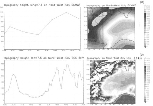
The GCRM performances were studied by considering one event of intense rain occured on November 2002 from 23th to 26th in Piemonte, a region in the Northwestern part of Italy. Piemonte is a predominantly alpine region, of about 25000 km , situated on the Padania plain and bounded on three sides by mountain-chains covering 73% of its territory (figure 1).

One problem to well forecast the meteorological calamitous in this area is due to its complex topography in which steep mountains and valleys are very close to each other (figure 2). In the event investigated, the precipitation exceeded 50 mm/24 hours over a vast Alpine area, with peaks above 100 mm over Northern Piemonte and also 150 mm in the South-Eastern Piemonte (figure 3).

3 Characteristic of numerical model and performed runs
A very special topic of the GCRM is the Yin-Yang grid system, characterized by two partially overlapped volume meshes which cover the Earth surface. One grid component is defined as part of the low-latitude region between 45N and 45S, extended for 270 degrees in longitude of the usual latitude-longitude grid system; the other grid component is defined in the same way, but in a rotated spherical coordinate system (ffigure 4)[10].

The upper surface of both meshes is located 30000 m above sea level. The flow equations for the atmosphere are non-hydrostatic and fully compressible, written in flux form [11]. The prognostic variables are: momentum, and perturbation of density and pressure, calculated with respect to the hydrostatic reference state. Smagorinsky-Lilly parameterization for sub-grid scale mixing, and Reisner scheme for cloud microphysics parameterization are used. A simple radiation scheme is adopted. The ground temperature and ground moisture are computed by using a bucket model as a simplified land model. No cumulus parameterization scheme is used, with the hypothesis that the largest part of the precipitation processes is explicitly resolved with a 5.5 km grid resolution*. Silhouette topography is interpolated to 5.5 km from the 1 km USGS Global Land One-kilometer Base Elevation (GLOBE) terrain database. In the GCRM, as in LAMI, the influence of the wave drag on upper tropospheric flow is explicitly resolved. The GCRM programming language is Fortran90. On Earth Simulator (ES) 640 NEC SX-6 nodes (5120 vector processors) are available. The runs were performed using 192 nodes for a configuration with 32 vertical layers; the elapsed time for each run was about 6 hours. For each ran the forecast time was 36 hours.
A particular hybrid model of parallel implementation is used in this software code; the parallelism among nodes is achieved by MPI or HPF, while in each node microtasking or OpenMP is used. The theoretical peak performance using 192 nodes is about 12 TFlops, while the resulting sustained peak performance is about 6 TFlops; this means that the overall system efficiency is 48.3 %
4 The spin up
Since observation data are not incorporated into this version of GCRM, some period is required by the model to balance the information for the mass and wind fields, coming from the initial data interpolated by analysis* (data from Japan Meteorological Agency, JMA). This feature gives rise to spurious high-frequency oscillations of high amplitude during the initial hours of integration. This behaviour is called “spin up”. For GCRM the spin up is also amplified because the precipitation fields (graupel, rain and snow) are set to zero at initial time. A more accurate interpolation and a reduction of the “spin up” phenomenon should be obtained by using a small ratio between the horizontal resolution of the analysis (data to initialize the model run) and of the model one. In our test cases the horizontal resolution of the analysis is 100 km while the GCRM resolution is 5,5 km (in some test cases also 11 km was used). Test performed with similar meteorological models have shown that a good resolution ratio is between 1:3-1:6 [12] [13]. The spin up “window” occurs for 6 to 12 hours (in the forecast time) after initialization; in order to avoid spin up problems the compared results are obtained by cumulating QPF data on 24 hours, beginning from +12 to +36 forecasts hours, then the first 12 hours of forecast are not reliable.
Without a sufficiently long spin-up period the output data may contain, as verified in our runs, strange transient values of QPF. In particular one typical spin up problem, consisting in an erroneous structure of rainfalls (with “spot” of rain maxima), has been identified in the runs performed.
4 Analysis of model performances
4.1 Visual verification forecast
The data verification is qualitative and has been obtained by the so-called called “visual” or “eyeball” technique. This simply consists in the comparison between a map of forecast and a map of observed rainfall. This technique can also be applied to other meteorological variables as geopotential, relative humidity, wind and so on; but in these last cases it is necessary to compare the forecast maps with the analysis because no observation maps are available. As it will be demonstrated, also if this is a subjective verification, an enormous amount of useful information can be gained by examination of maps.
4.2 Results of the reference version
In the figure 5 has the forecast map of QPF obtained by the reference configuration, hereinafter CTRL is presented.

Comparing the forecast (figure 5) with the observed map (figure 3) is clear that there is a general underestimation over mountain areas, and a weak overestimation on the central lowlands. The three QPF components, rain, graupel* and snow are shown in figure 6. The analysis of these maps is very useful to understand the main cause of the rain underestimation. The forecasted values of snow and graupel are not realistic as it is possible to understand looking at Milan skew diagram*(figure 7)


The height of the freezing level was constantly increasing for the long duration of the southerly flow. The mean value over North-Western Italy was around 1900 meters on Saturday 23rd, and increased to 2600 meters on Tuesday the 26th. A further increase up to 2900 meters was registered the day after. This means, as observed by ground stations, that in this event only rain precipitation was present. This overestimation of graupel and snowfall can aexplain the underestimation of the forecasted amount of rain.
4.3 Tuning of some parameters that define the property of the air
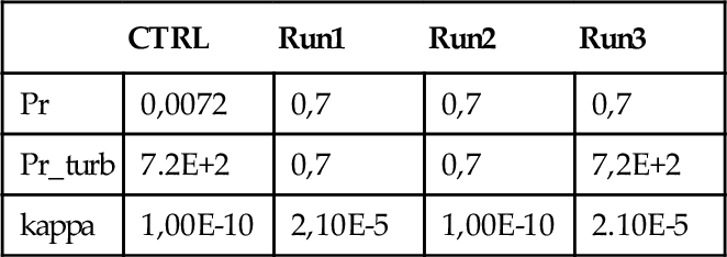
In the GCRM the Prandtl and the turbulent Prandtl numbers are used. The first one is defined among the properties of planetary boundary layer; the second one is used to characterize the properties of horizontal and vertical turbulent fluxes (using Smagorinsky-Lilly scheme). The value of the Prandtl number (hereinafter Pr) is defined by the fluid chemical composition and by its state (temperature and pressure), and is about 0.7 in the atmosphere. The turbulent Prandtl number (hereinafter Pr_turb) is defined by coefficients that are not air physical properties, but functions of flow and numerical grid characteristics. The turbulent Prandtl number depends on the horizontal numerical resolution and changes with the turbulence. In the reference version of the GCRM the Prandtl and the turbulent Prandtl numbers are set to the same value. Some runs to evaluate the model sensitivity to these two parameters has been performed [18]. The sensitivity to the thermal diffusivity (kappa) has also been checked. A Significant sensitivity was found. In particular the rain precipitation over the Mediterranean sea and over the southern coast (where the maximum was located) seems to be quite influenced by these parameters (figure 8).

5 Future developments
5.1 The microphysical schemes
The test cases performed by GCRM have shown a systematic overestimation of graupel and snow fall. This overestimation is one of the main cause of the strong underestimation of forecasted amount of rain.
The results obtained underline the necessity to improve the Reisner parameterization in GCRM. This sluod allow to obtain a better forecast of QPF. The Reisner explicit bulk mixed-phase model for microphysical parameterization consists (version used in GCRM) in five prognostic variables: water vapour mixing ratio (qv), cloud water mixing ratio (qc), rain water mixing ratio (qr), cloud ice mixing ratio (qi), snow mixing ratio (qs), graupel mixing ratio (qg), number concentration of cloud ice (Ni), number concentration of snow (Ns), number concentration of graupel (Ng) (figura 9). It is known from the literature that this scheme [15] has some overprediction of snow and graupel amount. Other teams developing meteorological models (as WRF model [16]), that previously used the Reisner parameterization, decided to upgrade the Reisner model following Thompson [17]. The principal improvements the replacement of primary ice nucleation and of auto-conversion formula, a new function for graupel distribution, and other corrections about formation of snow, rain and graupel.
5.2 The vertical grid system
Currently 32 vertical levels, defined by using the Gal-Chen terrain-following vertical-coordinate [19], are used in the reference version of GCRM, The top level is fixed at 30000 m (12 hPa in standard atmosphere). For meteorological models in which the upper boundary is supposed to be a rigid lid, the best choice, in order to avoid the spurious reflections of gravity waves, is 0 hPa; nevertheless this requirement is computationally quite expensive. A good compromise for the height-top in the global model is around 10 hPa for standard atmosphere (as ECMWF with 63 model levels [20]). Furthermore, to improve the representation of the near-bottom flow, it is necessary to increase the amount of vertical levels in the lower part of the troposphere (the bottom of the physical domain). This is useful especially in steep areas, as those involved in our test cases. This feature also requires an high computational cost. Looking at the literature, for meteorological model with a horizontal resolution of about 5-10 km, a good choice for the lowest level height is 40-80 m.
Taking into account all these considerations better results could be obtainded increasing the number of vertical level.
Acknowlegment
The authors wish to thank all the meteorological staff of the Environment Protection Regional Agency of Piedmont (ARPA) for having provided the data and maps and for help and support.