1 Introduction

The turbulent Poiseuille or Couette-Poiseuille flows inside a square or rectangular cross-sectional duct are of considerable engineering interest because their relevance to the compact heat exchangers and gas turbine cooling systems. The most studied flow is the turbulent Poiseuille type inside a square duct and is characterized by the existence of secondary flow of Prandtl’s [1] second kind which is not observed in circular ducts nor in laminar rectangular ducts. The secondary flow is a mean circulatory motion perpendicular to the streamwise direction driven by the turbulence. Although weak in magnitude (only a few percent of the streamwise bulk velocity), secondary flow is very significant on the momentum and hear transfer.

Fukushima and Kasagi [2] studied turbulent Poiseuille flow through square and diamond ducts and found different vortex pairs between the obtuse-angle and acute-angle corners in the diamond duct. A pair of larger counter-rotating vortices presented near the corners of acute-angle with their centers further away from the corner. Heating at the wall in a square duct was found to have evident effect on the secondary flow structure as well ([3] [4] [5]). Salinas-Vázquez and Métais [5] simulated a turbulent Poiseuille flow in a square duct with one high temperature wall and observed that the size and intensity of secondary flow increase in tandem with the heating. At the corner with heated and non-heated walls, there; exhibited a non-equalized vortex pair where vortex near the heated wall is much larger than the other. The combined effects of the bounding wall geometry and heating on the secondary flow in a non-circular duct is studied by Salinas-Vázquez et al. [6]. By computing the heated turbulent flow through a square duct with one ridged wall, new secondary flows were revealed near the ridges. Rotation around an axis perpendicular to the streamwise flow direction was also found to greatly modify the secondary flow structure in a LES calculation conducted by Pallares and Davidson [7]. The above investigations have implied that, with careful manipulation, the secondary flow is very much promising on enhancement of particle transport or single phase heat transfer in different industrial devices. They also demonstrated that the turbulence generated secondary flow in non-circular ducts could be modified by bounding wall geometry, heating and system rotation.

However, little is known about the effect of the moving wall on the secondary flow structure. Lo and Lin [8] investigated the Couette-Poiseuille flow with emphasis on the mechanism of the secondary flow vorticity transport within the square duct. However, the relationship between the secondary flow structure and the moving wall is not addressed. In the present study, focus is directed to the influences of the moving wall on the secondary flow pattern and hence turbulence structure.

2 Governing Equations and Modeling

The governing equations are grid-filtered, incompressible continuity and Navier-Stokes equations. In the present study, the Smagorinsky model[9] has been used for the sub-grid stress(SGS).

τsij=−(CsΔ)212√(SklSkl)−−−−−−√Sij+23ρksgsδij${\tau }_{ij}^s=-{\left(C_s\text{Δ}\right)}^2\frac{1}{\sqrt{2}}\sqrt{\left(S_{kl}{S}_{kl}\right)}{S}_{ij}+\frac{2}{3}\rho k_{sgs}{\delta }_{ij}$${\tau }_{ij}^s=-{\left(C_s\text{Δ}\right)}^2\frac{1}{\sqrt{2}}\sqrt{\left(S_{kl}{S}_{kl}\right)}{S}_{ij}+\frac{2}{3}\rho k_{sgs}{\delta }_{ij}$

where $C_s=0.1,S_{ij}=\frac{\partial {\overline{\mu }}_i}{\partial x_j}+\frac{\partial {\overline{\mu }}_j}{\partial x_i}$, and Δ=(ΔxΔyΔz)^1/3 is the length scale. It can be seen that in the present study the mesh size is used as the filtering operator. A Van Driest damping function accounts for the effect of the wall on sub-grid scales is adopted here and takes the form as, $l_m=\kappa y[1-exp(-\frac{y^4}{25})]$, where y is the distance to the wall and the length scale is redefined as, $\text{Δ}=Min[l_m,{\left(\text{Δ}x\text{Δ}y\text{Δ}z\right)}^{1/3}]$. Although other models which employed dynamic procedures on determining the Smagorinsky constant (C_s) might be more general and rigorous, the Smagorinsky model is computationally cheaper among other eddy viscosity type LES models. Investigations carried out by Breuer and Rodi [10] on the turbulent Poiscuille flow through a straight and bent square duct have indicated that, the difference between the predicted turbulence statistics using dynamic models and Smagorinsky model was only negligible.

3 Numerical and parallel Algorithms

A semi-implicit, fractional step method proposed by Choi and Moin [11] and the finite volume method are employed to solve the filtered incompressible Navier-Stokes equations. Spatial derivatives are approximated using second-order central difference schemes. The non-linear terms are advanced with the Adams-Bashfoth scheme in time, whereas the Crank-Nicholson scheme is adopted for the diffusion terms. The discretized algebraic equations from momentum equations are solved by the preconditioned Conjugate Gradient solver. In each time step a Poisson equation is solved to obtain a divergence free velocity field. Because the grid spacing is uniform in the streamwise direction, together with the adoption of the periodic boundary conditions, Fourier transform can be used to reduce the 3-D Poisson equation to uncoupled 2-D algebraic equations. The algebraic equations are solved by the direct solver using LU decomposition. In all the cases considered here the grid size employed is (128x128x96) m the spanwise, normal, and streamwise direction. respectively.

In the present parallel implementation, the single program multiple data (SPMD) environment is adopted. The domain decomposition is done on the last dimension of the three dimensional computation domain due to the explicit numerical treatment on that direction. The simulation is conducted on the IIP Integrity rx2600 server (192 Nodes) with about efficiency when 48 CPUs are employed in the compulation shown in Figure 2, Linear speed-up is not reached in present parallel implementation mainly due to the global data movement required by the Fast Fourier Transform in the homogenous direction.

4 Results

Schematic picture of the flows simulated is shown in Figure 1. where D is the duct width. We consider fully developed, incompressible turbulent Couette-Poiseuille flows inside a square duct where the basic flow parameters are summarized in Table 1. Reynolds number based on the bulk velocity (Re_bulk) is kept around 9700 for all cases simulated and the importance of Couette effect in this combined flow field can be indicated by the ratio r = (W_a/W_Bulk) and $-\frac{D}{p{W}_h^2}\frac{\partial P}{\partial z}$. Due to the lack of benchmark data of the flow filed calculated here, the simulation procedures were first validated by simulating a turbulent Poiseuille flow at a comparable bulk Reynolds number (case P). The obtained results (see Lo [12]) exhibit reasonable agreement with DNS data from Huser and Biringen [13].

Table 1

The flow conditions for simulated eases; Re_τ is defined by mean friction velocity averaged over four solid walls (t=top.b=bot,lom wall); W_w. denotes the velocity of the moving wall and W_Bulk, is the bulk velocity: ${Re}_c=\frac{W_{\omega }D}{v};r=\frac{W_{\omega }}{W_{Bulk}}$.

	Reτl	Reτb	Reτ	ReBulk	Rec	r	$-\frac{D}{\rho W_{\omega }^2}\frac{\partial P}{\partial z}$
Case P	600	600	600	9708	0	0	∞
Case CP1	441	605	571	9716	4568	0.47	0.0621
Case CP2	305	591	538	9760	9136	0.94	0.0138
Case CP3	284	587	533	9770	11420	1.17	0.0083
Kuroda et al. (1993)	35	308	172	5178	6000	1.16	0.0026

4.1 Mean secondary flow structure

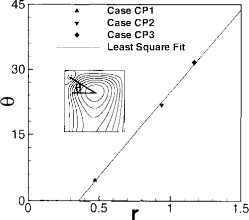
Streamlines of mean secondary flow are shown in Figure 3. The vortex structure is clearly visible, where solid and dashed lines represents counter-clockwise and clockwise rotation, respectively. The two clockwise rotating vortices are observed to gradually merge in tandem with moving wall velocity. Focus is directed to the top vortex pair which consists of a small and a larger vortex. Examination of the vortex cores by the streamline contours indicates that the distance between the vortex cores of vortex pair is approximately constant. Therefore, the angle formed by the horizonal x axis and the line joining the two vortex cores might become a good representation of the relative vortex positions. This angle is calculated and plotted against the parameter r defined by W_a/W_bulk which can be interpreted as the non-dimensional moving wall velocity. It is interesting to note that a linear relation exits between the angle and the parameter r, as shown in Figure 4. The least square fit. of the simulation data reveals a relation of Θ = −13.56 + 38.26r.

4.2 Turbulence intensities

Figures 5(a)-(c) show the cross-plane distributions of the resolved turbulence kinetic energy. The distribution shows locally maximum near the stationary wall. Near the moving wall, on the other hand, turbulence level is greatly reduced by the insufficient. mean shear rate which is caused by the moving wall. The distribution of the turbulence kinetic energy near the top and bottom corners are highly related to the presence of mean secondary flow which has been revealed in Figure 3. Near the bottom corner high turbulence kinetic energy is been convected into the corner. Near the top corner, on the other hand, high turbulence kinetic energy generated near the side wall has been convected into the core region of the duct horizontally. The predicted normal Reynolds stresses and primary shear stress profiles normalized by the plane average friction velocity at bottom wall along wall-bisector (x/D = 0.5) are given in Figure 5(d). Here, the DNS data of plane Couettc-Poiseuille (r=1.16. Kuroda et al. [14]) flows and plane channel flows (Moser et al. [15]) are also included for comparisons. The r value of the plane Couette-Poiseuille flow is close to 1.17 of case CP3. Near the stationary wall, it is not surprising to observe that predicted turbulence intensities are similar of all cases considered, indicating that the influence of moving wall is not significant. On the contrary, near the top moving wall, gradual reductions of turbulence are predicted in tandem with the increase of the moving wall velocity. The profiles in the plane Couette-Poiseuille flow of Kuroda et al. [14] also show this differential levels and agree with present results for case CP2 and CP3, where the operating levels of r are similar. Near the stationary wall (y/D < 0.05), < v’w’ > appears to be unaffected by the moving wall. The gradients of the < v’w’ > of case CPs in the core region are less than case P and the position of < v’w’ >= 0 are shifted toward the moving wall. The same behaviors were found in the experimental study of Thurlow and Klewicki [16] and they concluded that the position of zero Reynolds shear stress would shift to the lower stress wall if the wall stresses in a channel are not symmetric. The shifting of the zero Reynolds stress location implies that there arc stronger vertical interactions of fluctuations across the duct center.

4.3 Anisotropy invariant map

The above discussion has revealed that the turbulence inside the turbulent Couettc-Poiseuille duet flows is very anisotropic. The anisotropy invariant map (AIM) is introduced here in order to provide more specific description of the turbulence structures. The invariants of the Reynolds stress tensors arc defined as II = −(l/2)b_ijb_ji ,III = (1/3)b_ijb_jkb_ki and $b_{ij}=<{u\prime }_i{u\prime }_j>/<{u\prime }_k{u\prime }_j>-1/3{\delta }_{ij}$. A cross-plot of −II versus III forms the anisotropy invariant map (AIM). All realizable Reynolds stress invariants must lie within the Lumley triangle [17]. This region is bounded by three lines, namely two component state, −II = 3(III+1/27), and two axi-symmetric states, III = ±(−II/3)^3/2. For the axi-symmetric states, Lee and Reynolds [18] described the positive and negative III as disk-like and rod-like turbulence, respectively. The intersections of the bounding lines represent the isotropic, one-component and two-component axi-symmetric states of turbulence. An demonstration of the Lumley triangle [17] is given in Figure 6.

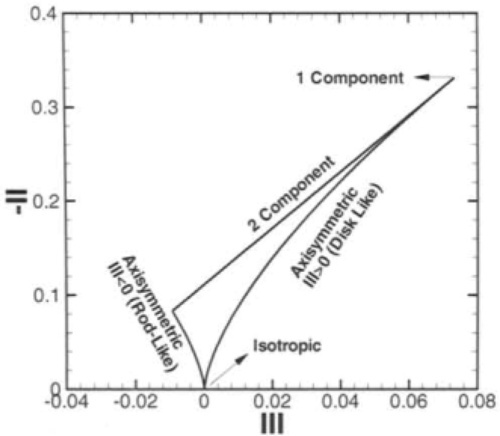
The AIM at two horizonal locations across the duct height is presented in Figure 7. Near the stationary wall (y/D ≤ 0.5), turbulence behaviors of different Couette-Poiseuille flows resemble those of the Poiseuille flow. In particular, along x/D=0.5, the turbulence structure is similar to the plane channel flow, where turbulence approaches two-component state near the stationary wall due to the highly suppressed wall-normal velocity fluctuation (Moser et al. [15]). It moves toward the one-component state till y⁺ ~ 8 (Salinas-Vázquez and Métais [5]) and then follows the positive 777 axi-symmetric branch (disk-like turbulence, Lee and Reynolds [18]) to the isotropic state at the duct center. However, near the moving wall due to the reduction of the streamwise velocity fluctuation at the moving wall, turbulence structure gradually moves towards a rod-like axi-symmetric turbulence (negative III) as r increases. It should be noted that for case CP2 and CP3. turbulence close to the top wall at x/D=0.5 has reached the two-component axi-symmetric state. The invariant variations of the case CP3 are similar to the plane Couette-Poiseuille flow of Kuroda et al. [14]. though the latter case is at a lower Reynolds number and therefore the isotropic state is not reached at the center of the channel. Comparison between AIM at x/D=0.5 from case CP1 to CP3 reveals that the anisotropy near the moving wall reduces with the wall velocity increased. At x/D=0.2 the turbulence is influenced by the side wall and deviates from the plane channel flow behavior near the stationary wall. where at y/D=0.5 the isotropic state is not reached. It is also noted that the difference between turbulence anisotropy near the stationary and moving wall is most evident at wall-bisector.

5 Conclusion

The turbulent Couette-Poiseuille (lows inside a square duct are investigated by present simulation procedures. Mean secondary flow is observed to be modified by the presence of moving wall where the symmetric vortex pattern vanishes. Secondary flow near the top corner shows a gradual change of vortex size and position as the moving wall velocity increased. The vortex pair consists of a dominate (clock-wise) and relatively smaller (counter-clockwise) vortex. For the three r considered, the relative positions of vortex cores have a linear dependence with r, which offers an easy estimation of the secondary (low structure. In addition, distance between the vortex cores of each vortex pair is also observed to remain approximately constant.

The turbulence level near the moving wall is reduced compared to other bounding walls which is caused by the insufficient mean shear rates. The distribution of the turbulence kinetic also demonstrated that the capability of mean secondary flow on transporting energy on the cross-plane of the square duct. The reductions of turbulence intensities along the wall-bisector are found to be similar with Kuroda et al. [14] when the operating value of r is comparable.

The anisotropy invariant analysis indicates that along the wall bisector at the top half of the duct, turbulence structure gradually moves towards a rod-like axi-symmetric state (negative III) as the moving wall velocity increased. It is observed that the turbulence anisotropy level is reduced along the wall-bisector near the moving wall. On the other hand, the anisotropy states near the bottom stationary wall resemble those presented in turbulent channel flow or boundary layers. The difference between turbulence anisotropy near the stationary and moving wall is most evident at wall-bisector.

6 Acknowledgments

This research work is supported by the National Science Council of Taiwan under grant 95-2221-E-007 -227 and the computational facilities are provided by the National Center for High-Performance Computing of Taiwan which the authors gratefully acknowledge.