1 Motivation of Time Decomposition in the Parallel CFD context

Time domain decomposition methods can bo a complementary approach to improve parallelism on the forthcoming parallel architectures with thousand of processors. Indeed. for a given modelled problem. e.g. through a partial differential equation with a prescribed discretization- the multiplication of the processors leads to a decrease of the computing load allocated to each processors, then the ratio of the computing time with the communication time decreases, leading to less efficiency. Nevertheless, for the evolution problems, the difficulty comes from the sequential nature of the computing. Previous time steps are required to compute the current time step. This last constraint occurs in all time integrators used in computational fluid dynamics of unsteady problems.

During these last years, some attempts have been proposed to develop parallelism in time solvers. Such algorithms as Parareal [6] or Pita [2] algorithms are multiple shooting type methods and are very sensitive to the Jabobian linearization for the correction stage on stiff non-linear problems as shown in [4].

Moreover, this correction step is an algorithm sequential and often much more time consuming to solve for the time integrator than the initial problem.

In this paper we investigate a new solution to obtain a parallelism in time with a two level algorithm that combines pipelined iterations in time and deferred correction iterations to increase the accuracy of the solution. In order to focus on the benefit, of our algorithm we approach CFD problems as an ODE (eventually DAE) problem. From the numerical point of view the development of time domain decomposition methods for stiff ODE problems allows to focus on the time domain decomposition without perturbation coming from the space decomposition. In other side, classical advantages of the space decomposition on the granularity are not available. Indeed, from the engineering point of view in the design with ODE/DAE. the efficiency of the algorithm is more focus on the saving time in the day to day practice.

2 ODE approach for CFD problem

The traditional approach to solve CFD problems starts from the partial differential equation, which is discretized in space with a given accuracy and finally a time discretization with a first order scheme or a second order time scheme is performed to solve problems (usually implicitly due to Courant-Friedrich-Lax condition constraint).

Let consider the 2D Navier-Stokes equations in a Stream function - vorticity formulation:

$\{\begin{array}{c}\begin{array}{c}{\omega }_t+{\psi }_x{\omega }_y-{\psi }_y{\omega }_x-\frac{1}{Re}\text{Δ}\omega =0\\ \text{Δ}\psi =-\omega \end{array}\\ \psi =0,{\psi }_n=v\left(t\right)\text{on}\partial \mathrm{\Omega }\end{array}$

then applying a backward (forward Euler or Runge-Kutta are also possible) time discretisation. we obtain that follows:

$\{\begin{array}{c}{\omega }^{n+1}+{\text{Δ}}_t({\psi }_x^n{\omega }_y^{n+1}-{\psi }_x^n{\omega }_y^{n+1})-\frac{\text{Δ}t}{Re}\text{Δ}{\omega }^{n+1}={\omega }^n\\ \text{Δ}{\psi }^{n+1}=-\text{Δ}{\omega }^{n+1}\end{array}$

The discretization in space of the discrete in time equations leads to solve a linearized system with an efficient preconditionned solver such as Schwarz-Krylov method or multi-grid:

$\{A\left({\psi }^n\right){\omega }^{n+1}=f\left({\psi }^n\right),\text{Δ}{\psi }^{n+1}=-{\omega }^{n+1}$

Let us consider an another approach that is the method of lines or ODE to solve CFD problems. Firstly, the Navier-Stokes problem is written in a Cauchy equation form:

$\frac{d}{dt}\left(\begin{array}{c}\omega \\ \psi \end{array}\right)\left(t\right)=f(t,\omega ,\psi ),\left(\begin{array}{c}\omega \\ \psi \end{array}\right)\left(0\right)=\left(\begin{array}{c}{\omega }_0\\ {\psi }_0\end{array}\right)$

then the discretization in space of the f(t, ω, ψ) leads to a system of ODE:

$\frac{d}{dt}\left(\begin{array}{c}{\omega }_{i,j}\\ {\psi }_{i,j}\end{array}\right)=f(t,{\omega }_{i[\pm 1],j[\pm 1]},{\psi }_{i[\pm 1],j[\pm 1]})$

This last equation can be solved by an available ODE solver such as SUNDIALS (SUite of Nonlinear and Differential/ALgebraic equation Solvers (http://www.llnl.gov/casc/sundials/)) that contains the latest developments of classical ODE solvers as LSODA [8] or CVODE [1]

Figure 1 corresponds to the lid driven cavity results computed by the ODE method a Reynold number of 5000 and up to 10000. These results are obtained for the impulse lid driven with a velocity of 1. Let us notice that the convergence is sensitive to the singularities of the solution.

The advantages and drawbacks of the PDEs and ODE are summarized in Table 1

In conclusion the ODE approach put the computing pressure on the time step control while PDEs approach put the computing pressure on the preconditionned linear/nonlinear solver.

The high time consumming drawback for ODE explains why this approach is not commonly use in CFD. Nevertheless grid computing architecture could give a renewed interest to this ODE approach.

3 Spectral Deferred Correction Method

The spectral deferred correction method (SDC) [7] is a method to improve the accuracy of a time integrator iteratively in order to approximate solution of a functional equation with adding corrections to the defect.

Let us summarize the SDC method for the Cauchy equation:

$y\left(t\right)=y_0+{\int }_0^{1}f(\tau ,y\left(\tau \right))d\tau$

Let $y_m^0\simeq y\left(t_m\right)$ an approximation of the searched solution at time t_m. Then consider the polynomial q₀ that interpolate the function f(t,y) at P points ${\tilde{t}}_i$ i.e:

$\exists !q_0\in R_p\left[x\right],q_0\left({\tilde{t}}_i\right)=f\left(y^0\right({\tilde{t}}_i\left)\right)$

with $\{{\tilde{t}}_0<{\tilde{t}}_1<\dots <{\tilde{t}}_p\}$ are points around t_m. Then if we define the error between the approximate solution $y_m^0$ and the approximate solution using q₀:

$E(y^0,t_m)=y_0+{\int }_0^{t_m}{q}^0\left(\tau \right)d\tau -y_m^0$

Then we can write the error between the exact solution and the approximation $y_m^0$:

$y\left(t_m\right)-y_m^0={\int }_0^{t_m}\left(f(\tau ,y\left(\tau \right))+q^0\left(t\right)\right)d\tau +E(y^0,t_m)$

The defect $\delta \left(t_m\right)=y\left(t_m\right)-y_m^0$, satisfies:

$\delta \left(t_{m-1}\right)=\delta \left(t_m\right)+{\int }_{t_m}^{t_{m+1}}\left(f(\tau ,y^0\left(\tau \right)+\delta (\tau \left)\right)+q^0\left(\tau \right)\right)d\tau +E(y^0,t_{m+1})-E(y^0,t_m)$

For the spectral deferred correction method an approximation ${\delta }_m^0$ of δ(t_m) is computed considering for example a Forward Euler scheme:

${\delta }_{m+1}^0={\delta }_m^0+{\text{Δ}}_t\left(f(t_{m+1},y_{m+1}^0+{\delta }_{m+1}^0)-f(t_{m+1},y_{m+1}^0)\right)-y_{m+1}^0+y_m^0+{\int }_{t_m}^{t_{m+1}}{q}^0\left(\tau \right)d\tau$

Once the defect computed, the approximation $y_m^0$ is updated

$y_m^1=y_m^0+{\delta }_m^0\mathrm{.}$

Then a new q₀ is computed with using the value $y_m^1$ for a new iterate. This method is a sequential iterative process as follows: compute an approximation y⁰, then iterate in parallel until convergence compute δ and update the solution y by adding the correction term δ.

We propose in the next section a parallel implementation to combine deferred correction method with time domain decomposition.

4 Parallel SDC: a time domain decomposition pipelined approach

The main idea to introduce parallelism in the SDC is to consider the time domain decomposition and to affect a set of time slices to each processors. Then we can pipeline the computation, each processor dealing a different iterate of the SDC.

Table 2 gives the times to run the timo domain decomposition pipelined SDC method on an ALTIX350 with IA64 1.5Ghz/6Mo processors and with numalink communication network. The lid driven parameters are a Reynolds number of 10 and a regular mesh of 20 × 20 points, the final time to be reach is T=5. The number of time slices has been set equal to 805. The number of SDC iteration is 25. The stage [1] correspond to the sequential first evaluation of the solution on the time slices (with an rtol of 10⁻¹). The time [2.2] is the time of the pipelined to reach the last processor, results show that the ratio of this time [2.2] on the computation is increasing up to 1/4 for 8 processors case. The Speed-up corrected line gives the parallel capability of the parallel implementation when the pipeline is full.

It exhibits quite reasonable speed-up up to 8 processors for the present implementation.

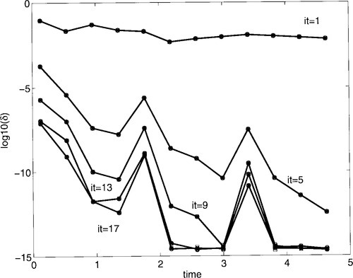
Figure 2 gives the convergence of the defect on the time interval for different iteration numbers (1.5.9,13,17). Symbols represent the runs on 1 processor (x). 2 processors (o). 8 processors (). Firstly, we remark that the number of processors does not impact the convergence properties of the method. Secondly, the convergence behavior increases for the last times due to the steady state of the solution. Nevertheless, a good accuracy is obtained on the first times in few SDC iterates.

5 conclusions

In this work we have investigated the numerical solution of 2D Navier-stokes with ODE solvers in the perspective of the time domain decomposition which can be an issue for the grid computing.

we proposed to combine time domain decomposition and spectral deferred correction in order to have a two level algorithm that can be pipelined. The first results proved some parallel efficiency with a such approach.

Nevertheless, the arithmetical complexity of the ODE solver for the lid driven problem consider here, is too much costly. Some scheme such as the C(p, q, j) [3] schemes can decouple the system variables in order to reduce the complexity.