
Chapter 26. Sound
In this chapter we’ll explore some basic physics of sound and how you can capture 3D sound effects in games. We’ll refer to the OpenAL audio API for some code examples, but the physics we discuss is independent of any particular API. If you’re new to OpenAL, it’s basically OpenGL for audio. OpenAL uses some very easy-to-understand abstractions for creating sound effects and handles all the mixing, filters, and 3D synthesis for you. You basically create sound sources, associate those sources with buffers that store the sound data, and then manipulate those sources by positioning them and setting their velocity (among other properties). You can have multiple sources, of course, but there’s only one listener. You do have to set properties of the listener, such as the listener’s position and velocity, in order to properly simulate 3D sound. We’ll talk more about these things throughout the chapter.
What Is Sound?
If you look up the definition of sound online, you’ll get answers like sound is a vibration; a sensation perceived by our brains through stimulation of organs in our inner ear; and a density or pressure fluctuation, or wave, traveling through a medium. So which is it? Well, it’s all of them, and the interpretation you use depends on the context in which you’re examining sound. For example, noise control engineers aiming to minimize noise on ships focus on vibrations propagating through the ship’s structure, while medical doctors worry more about the biomechanics of our inner ear and how our brains interpret the sensations picked up by our ears, and physicists take a fundamental look at density and pressure fluctuations through compressible materials and how these waves interact with each other and the environment. We don’t mean to suggest that each of these disciplines views sound only in a single way or context, but what we’re saying is that each discipline often has its own perspective, priorities, and standard language for the subject. To us, in the context of games, sound is what the player hears through his speakers or headphones that helps to create an immersive gaming environment. However, in order to create realistic sounds that lend themselves to creating an immersive environment, complimenting immersive visuals and in-game behaviors, we need to understand the physics of sound, how we perceive it, and what sound tells us about its source and the environment.
Given that this is a book on game physics, we’re going to take a fundamental view of sound, which is that sound is what our brain perceives as our ears sense density and pressure fluctuations in the air surrounding us. These density and pressure fluctuations are waves, and as such we’ll refer to sound waves. Let’s take a closer look.
If a compressible medium experiences a pressure change—say, due to a driven piston—its volume will change and thus its density will change. In the case of a driven piston, the region directly in front of the piston will experience the compression first, resulting in a region of increased density and increased pressure. This is called condensation. For sound, you can think of that piston as the cone of a loudspeaker. That region of increased density and pressure will propagate through the medium, traveling at the speed of sound in that given medium. Figure 26-1 illustrates this concept.
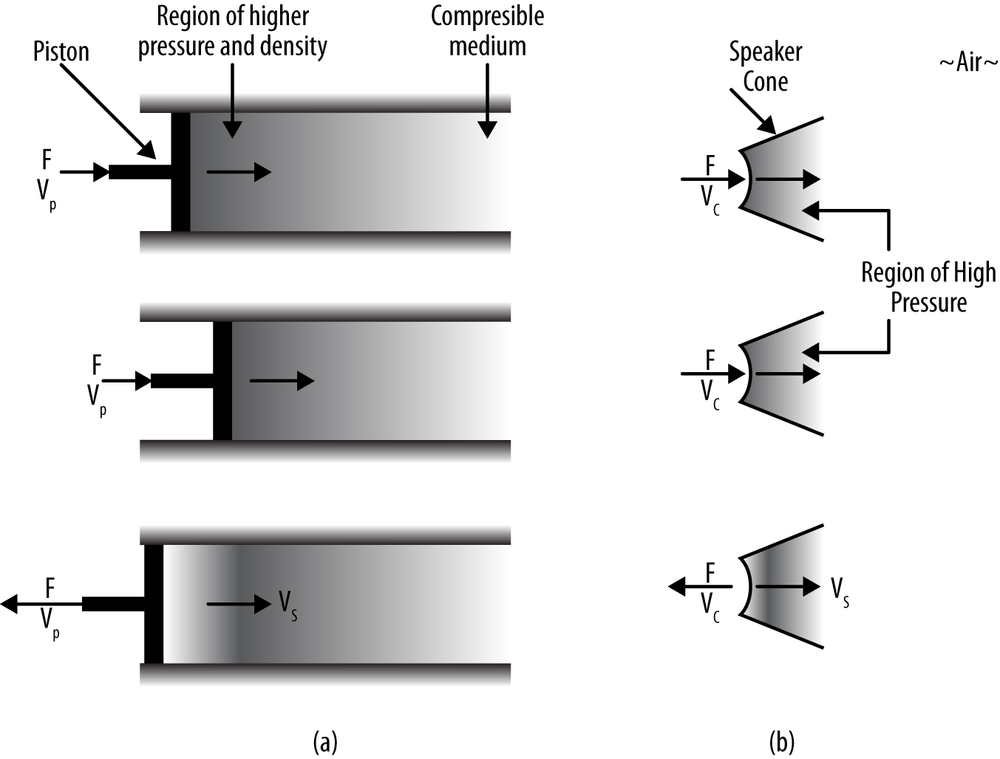
Figure 26-1(a) illustrates the driven piston concept, while Figure 26-1(b) illustrates the loudspeaker analogue. As the piston or cone displaces fluid (say, air), causing compression, and then withdraws, a single high-pressure region followed by a low-pressure region will be created. The low-pressure region resulting from withdrawal of the piston is called rarefaction. That resulting solitary wave of pressure will head off through the air to the right in Figure 26-1 at the speed corresponding to the speed of sound in air. If the piston, or speaker cone, pulses back and forth, as illustrated in Figure 26-2, a series of these high-/low-pressure regions will be created, resulting in a continuous series of waves—a sound wave—propagating to the right.
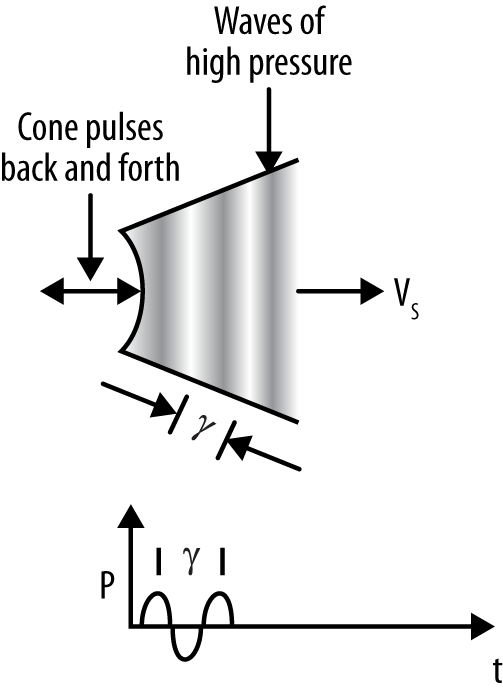
The wavelength of this sound wave (i.e., the distance measured from pressure peak to pressure peak) is a function of the frequency of pulsation, or vibration, of the cone. The resulting sound wave’s frequency is related to the inverse of its wavelength—that is, f = 1/λ. The pressure amplitude versus time waveform for this scenario is illustrated in Figure 26-2. We’ve illustrated the pressure wave as a harmonic sine wave, which need not be the case in reality since the sound coming from a speaker could be composed of an aggregate of many different wave components. We’ll say more on this later.
One thing we do want to point out is that a sound wave is a longitudinal wave and not a transverse wave like an ocean wave, for example. In a transverse wave, the displacement of the medium due to the wave is perpendicular to the direction of travel of the wave. In a longitudinal wave, the displacement is along the direction of travel of the wave. The higher density and pressure regions of a sound wave are due to compression of the medium along the direction of travel of the wave. Thus, sound waves are longitudinal waves.
So, sound waves are variations in density and pressure moving through a medium. But how do we hear them? In essence the pressure wave, created by some mechanical vibration like that of a speaker cone, gets converted back to a vibration in our inner ear. And that vibration gets interpreted by our brains as sound—the sound we hear. Figure 26-3 illustrates this concept.
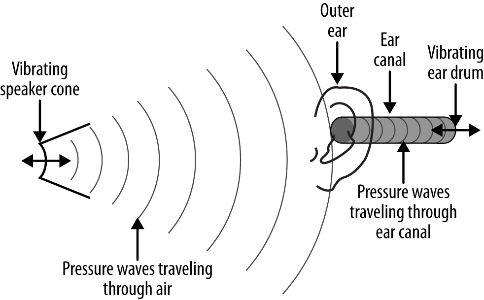
Our outer ears help capture and direct pressure waves into our ear canals. These pressure waves travel down the ear canal, impinging on the eardrum, which causes the eardrum to vibrate. This is where the pressure variations get converted back to mechanical vibration. Beyond the eardrum, biology and chemistry work their magic to convert those vibrations into electrical impulses that our brains interpret as sound.
Our ears are sensitive enough to detect pressure waves in the 20 to 20,000 hertz (Hz) frequency range. (A hertz is one cycle per second.) We interpret frequency as pitch. High-pitch sounds (think tweeters) correspond to high frequencies, and low-pitch sounds (think bass) correspond to low frequencies.
Aside from pitch, an obvious characteristic of sound that we perceive is its loudness. Loudness is related to the amplitude of the pressure wave, among other factors such as duration. We often think of loudness in terms of volume, or power, or intensity. All these characteristics are related, and we can write various formulas relating these characteristics to other features of the sound wave. Sound waves have kinetic energy, which is related to the mass of the medium disturbed by the pressure wave and the speed at which that mass is disturbed. Power is the time rate of change of energy transference. And intensity is related to how much power flows through a given area. The bottom line is that the more power a sound has, or the more intense it is, the louder it seems to you, the listener. At some point, a sound can be so intense as to cause discomfort or pain.
Customarily, intensity is measured in units of decibels. A decibel represents the intensity of a sound relative to some standard reference, which is usually taken as the sound intensity corresponding to the threshold of hearing. Zero decibels, or 0 dB, corresponds to the threshold of hearing. The intensity is so low you can’t hear it. When sounds reach about 120–130 dB, they start to cause pain. Table 26-1 lists some typical intensity values for common sounds.
Sound | Typical intensity |
Jet airplane, fairly close | 150 dB |
Gun shot | 160 to 180 dB depending on the gun |
Crying baby | 130 dB (painful!) |
Loud scream | Up to 128 dB (world record set in 1988) |
Typical conversation | 50 to 60 dB |
Whisper | About 10 dB |
The intensity values shown in Table 26-1 are typical and surely there’s wide variation in those levels depending on, for example, the type of aircraft, or the person you’re talking to, or the softness of the person’s voice whispering to you. It’s common sense, but if you’re writing a game you’ll want to reflect some level of realism in the intensity of various sound effects in your game.
Now, intensity is actually a logarithmic scale. It is generally accepted that a sound measured 10 dB higher than another is considered twice as loud. This is perceived loudness. Thus, a crying baby is way more than twice as loud as a normal conversation. Parents already know that.
Characteristics of and Behavior of Sound Waves
Now that we’ve established what sound is, we’re going to generally refer to sound waves throughout the remainder of this chapter. Remember, sound waves are pressure waves that get interpreted by our brains as sound. The bottom line is that we’re dealing with waves, longitudinal waves. Therefore, we can use principles of wave mechanics to describe sound waves. Furthermore, since sound waves (think pressure waves) displace real mass, they can interact with the environment. We already know that pressure waves interact with our eardrums to trigger some biochemical action, causing our brains to interpret sound. Conversely, the environment can interact with the pressure wave to alter its characteristics.
Harmonic Wave
Let’s consider a one-dimensional harmonic pressure wave—one that could be created by the driven piston shown in Figure 26-1(a). Let the x-direction correspond to distance, positive from left to right. Thus, the wave of Figure 26-1(a) travels in the positive x-direction. Let ΔP represent the change in pressure from the ambient pressure at any given time. Let AP represent the amplitude of the pressure wave. Remember, the pressure will vary by some amount greater than the ambient pressure when condensation occurs to some amount lower than ambient pressure when rarefaction occurs. The range in peak pressures relative to ambient is −AP to +AP. Assuming a harmonic wave, we can write:
| ΔP = AP sin(kx – ωt – φ) |
k is called the wave number and is equal to 2π/λ, where λ is the wave length. x is the coordinate representing the position under consideration. ω is called angular, or circular, frequency and is equal to 2πf, where f is the frequency of the sound wave. t represents time. Finally, φ is called the phase angle, also known as the phase shift. It represents an offset of the wave along the x-axis in this case.
With this equation, we can plot what ΔP at a particular x-location as a function of time. Figure 26-4 illustrates such a plot assuming that AP, λ, and f are all equal to 1 and φ is equal to 0.
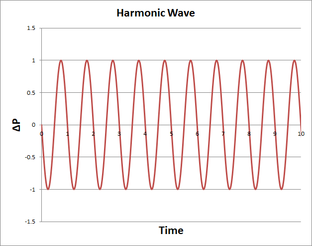
Physically, if you were to measure the change in pressure over time at some point, x, the plot would look like that shown in Figure 26-4.
Superposition
In general, sound waves don’t look like the pure harmonic wave shown in Figure 26-4 unless the sound is a pure tone. A non-pure tone will have other wiggles in its plot resulting from components at other frequencies and phases. Similarly, if you record the sound pressure at a single point in a room, for example, where multiple sound sources exist, the pressure recording at the point in question will not correspond to the sound of any particular sound source. Instead, the recorded pressure time history will be some combination of all the sources present, and what you hear is some combination of all the sound sources.
A good approximation for how these various sound components combine is simply to sum the results of each component at the particular point in question. This is the principle of superposition.
Figure 26-5 shows 10 different waveforms, each with different amplitudes, frequencies, and phases. The principle of superposition says that we can add all these waveforms to determine the combined result.
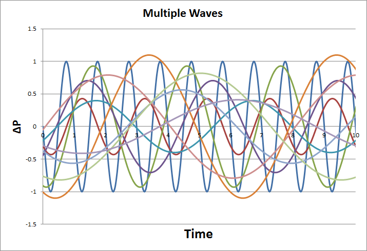
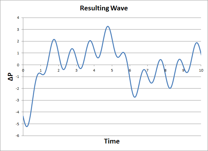
Figure 26-6 shows the resulting wave. Note that the individual waves are added algebraically. At any given instant in time, some waves produce positive pressure changes, while others produce negative pressure changes. This means that some waves add together to make bigger pressure changes, but it also means that some can add together to make smaller pressure changes. In other words, waves can be either constructive or destructive. Some waves can cancel each other out completely, which is the basis for noise cancellation technologies.
Speed of Sound
Sound waves travel through a medium at some finite speed, which is a function of that medium’s elastic and inertial properties. In general, sound travels faster in stiffer, less compressible mediums than it does in softer or more compressible mediums. For example, the speed of sound in air is about 340 m/s, depending on temperature, moisture content, and other factors, but it’s about 1500 m/s in seawater. Water is a lot less compressible than air. Taking this a step further, the speed of sound in a solid such as iron is about 5,100 m/s.
You might say, “So what; why do I have to worry about the speed of sound in my game?” Well, the speed at which sound waves travel tells us something about the sound source, and you can leverage those cues in your game to enhance its immersive feel. Let’s say an enemy unit fires a gun in your 3D shooter, and that enemy is some distance from your player. The player should see the muzzle flash before she hears the sound of the gun firing. This delay is due to the fact that light travels far faster than sound. The delay between seeing the muzzle flash and hearing the shot gives the player some sense of the distance from which the enemy is firing.
With respect to 3D sound effects, our ears hear sounds coming from an oblique direction at slightly different times because of the separation distance between our ears. That time lag, albeit very short, gives us some cues as to the direction from which the sound is coming. We’ll say more on this later on this chapter.
Additionally, the Doppler effect, which we’ll discuss later, is also a function of the speed of sound.
In OpenAL you set the desired sound speed using the alSpeedOfSound function, passing a single
floating-point argument representing the sound speed. The specified
value is saved in the AL_SPEED_OF_SOUND
property. The default value is 343.3, which is the speed of sound in air
at 20°C expressed in m/s.
Attenuation
Attenuation is the falloff in intensity of a sound over distance. Earlier we explained that sound intensity is related to how much power flows through a given area. Imagine a point sound source, which creates spherical pressure waves that propagate radially from the source. Figure 26-7 illustrates this concept.
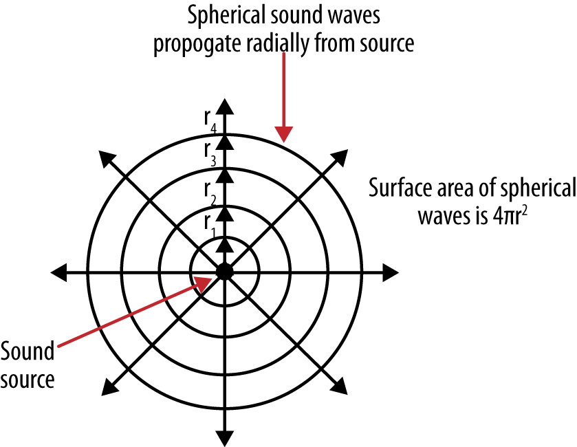
Assuming the sound is being generated with a constant power, you can see that the area through which that power flows grows with increasing distance, r, from the source. Intensity is equal to power divided by area, thus the intensity at radius r4 is less than that at, say, r1 because the surface area at r4 is larger. The surface area of a sphere is 4πr2. Without going into all the details, we can state that the amplitude of the spherical sound wave is inversely proportional to r2.
This is an ideal treatment so far. In reality attenuation is also a function of other factors, including the scattering and absorption of the sound wave as it interacts with the medium and the environment. You can model attenuation in many ways, taking into account various levels of detail at increasing computational expense. However, for games, relatively simple distance-based models are sufficient.
Attenuation provides another cue that tells us something about the sound source. In your game, you wouldn’t want the intensity, or volume, of a sound generated far from the player to be the same as that from a source very close to the player. Attenuation tells the player something about the distance between him and the sound source.
OpenAL includes several different distance-based models from which you can choose. The OpenAL documentation describes the particulars of each, but the default model is an inverse distance-based model where the gain of the source sound is adjusted in inverse proportion to the distance from the sound source. Gain is an amplification factor applied to the recorded amplitude of the sound effect you’re using.
You can change distance models in OpenAL using the alDistanceModel function (see the OpenAL
programmers manual for valid parameters).
Reflection
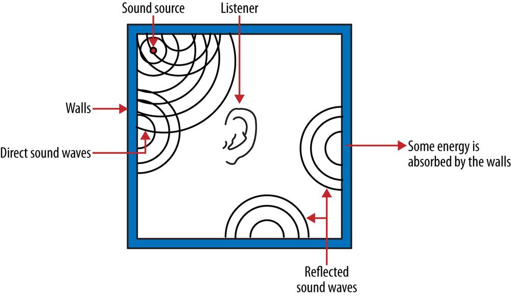
When sound waves passing through one medium reach another medium or object, such as a wall, part of the original sound wave is reflected off the object, while part of it is absorbed by (and transmitted through) the object. Depending on the dispositions of the sound source and the listener, some sound waves will reach the listener via some direct path. Reflected waves may also reach the listener, although their energy may have been reduced after their interaction with whatever they bounced off. Figure 26-8 illustrates this concept, where some sound waves reach the listener directly and others reach the listener after having been reflected from walls.
The degree to which sound waves are reflected has to do with the characteristics of the material from which they bounce. Smooth, hard surfaces will tend to reflect more of the sound energy, while softer, irregular surfaces will tend to absorb more energy and scatter the waves that are reflected. These characteristics lend a certain quality to the ultimate sound the listener hears. The same sound played in a tiled bathroom will have a distinctly different quality than if it were played in a room with carpet, drapes, and tapestries. In the bathroom the sound may sound echoic, while in the carpeted room it may sound muted. Somewhere in between these two types of rooms, the sound may reverberate. Reverberation is a perceived prolonging of the original sound due to reflections of the sound within the space.
In your games, it would be prohibitively expensive (computationally speaking) to try to model various sound sources interacting with all the walls and objects in any given space within the game in real time. Such computations are possible and are often used in acoustic engineering and noise control applications, but again, it’s too costly for a game. What you can do, however, is mimic the reflective or reverberant qualities of any given space in your game environment by adjusting the reverberation of your sound sources. One approach is to record sound effects with the quality you’re looking for to represent the space in which that sound effect would apply. For example, you could record the echoic sound of dripping water in a stone room to enhance the atmosphere of a dungeon.
Alternatively, if you’re using a system such as OpenAL and if the reverberation special effect is available on your sound card, you can assign certain reverberation characteristics to individual sound sources to mimic specific environments. This sort of approach falls within the realm of environmental modeling, and the OpenAL Effects Extension Guide (part of the OpenAL documentation) gives some pretty good tips on how to use its special effects extensions for environmental modeling.
Doppler Effect
The Doppler effect results when there is a relative motion between a sound source and the listener. It manifests itself as an increase in frequency when the source and listener are approaching each other, and a decrease in frequency when the source and listener are moving away from each other. For example, the horn of an approaching train seems to increase in pitch as it gets closer but seems to decrease in pitch as the train passes and moves away. The Doppler effect is a very obvious clue as to the relative motion of a sound source that you can capture in your games. For example, you could model the sound of a speeding car with a Doppler effect complimenting visual cues of a car approaching and passing by a player.
What’s happening physically is that the encounter frequency of the sound waves relative to the listener is augmented, owing to the relative velocity. An approaching velocity means there are more waves encountered by the listener per unit of time, which is heard as a higher frequency than the source frequency. Conversely, a departing velocity means there are fewer waves encountered per unit of time, which is heard as a lower frequency. Assuming still air, the increased frequency heard when the sound source and listener are approaching each other is given by the relation:
| fh = f [(c + vl)/(c + vs)] |
where fh is the frequency heard by the listener, c is the speed of sound, vl is the speed of the listener, and vs is the speed of the source. This equation shows that the frequency heard by the listener is increased in proportion to the ratio of the sum of the speed of sound plus the relative speed of the source and listener to the speed of sound. If the source and listener are moving away from each other, then vr is negative and the frequency heard is reduced.
For your game, you could use prerecorded sounds with Doppler effects for passing cars or other moving sound sources; however, you won’t be able to adjust the Doppler effect to represent the actual relative speed between sound source and listener if you’re simulating the object to which the sound is attached using the techniques discussed in this book. Your prerecorded sound is fixed. It may work just fine, by the way. That said, if you’re using an audio system such as OpenAL, you can use its built-in Doppler effect capabilities. Basically, if you’re simulating an object that’s generating a sound, you update its sound source to reflect the object’s velocity while at the same time updating the listener object to reflect the player’s velocity. OpenAL will handle the rest for you. We’ll show a simple example of this in the next section.
3D Sound
At one time not so long ago, “3D sound” was hyped as the next big thing. There’s no doubt that for a long time, game sound lagged far behind graphics capabilities. It’s also true that good 3D sound can compliment good visuals, helping to create a more immersive gaming environment. Unfortunately, a lot of early 3D sound just wasn’t that good. Things are getting better, though, and with the use of headphones and a good sound card, some amazing 3D sounds can be generated.
If used properly, 3D sound can give your player the sensation that sounds are coming from different distinct directions. For example, a shot fired from behind the player would be accompanied by the player hearing a gunshot sound as though it really were coming from behind. Such directional sound really adds to the immersive experience of a game.
How We Hear in 3D
3D sound—or more specifically, our ability to localize a sound—is the result of a complex interaction between the sound source and our bodies, not to mention the room or environment we happen to be in. Ignoring environmental interactions, Figure 26-9 illustrates how a sound wave interacts with one’s body.
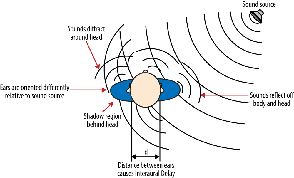
One of the first things you may notice is that our ears are separated by some finite distance. This means that the sound coming from the source on the right will reach the right ear before it reaches the left ear. The time delay between the sound reaching each ear is called the interaural delay. We can approximately calculate the delay from a sound coming from the side by taking the distance separating the ears and dividing it by the speed of sound. In air and for a typical head size, that delay is around half a millisecond. The delay will be shorter depending on the orientation of your head with respect to the sound source. Whatever the delay is, our brains use that information to help determine the location from which the sound is coming.
Additionally, as the sound coming from the right in Figure 26-9 reaches the head, some of the energy is reflected off the head. Reflections also occur off the shoulders and torso. Further, as the sound waves pass the head they tend to bend around it. Higher-frequency waves tend to get blocked by the head, and lower-frequency waves tend to pass by with little interruption. The resulting sound in the shadow region behind the head is somewhat different than the source due to the effective filtering that has occurred via interaction with the head. Also, notice that the orientation of the ears with respect to the sound source is different, and sound waves will interact with the ear and ear canal differently due to this differing orientation.
If the sound is coming from above or below the person in addition to being offset laterally, the sound will reflect off and diffract around different parts of the body in different ways.
Considering all these interactions, it would seem that the sound we end up hearing is quite different from the pure source sound. Well, the differences may not be that dramatic, but they are sufficient to allow our brains to pick up on all these cues, allowing us to locate the sound source. Given that we are all different shapes and sizes, our brains are tuned to our specific bodies when processing these localization cues.
It would seem that including believable 3D sound is virtually impossible to achieve in games given the complexity of sounds interacting with the listener. Certainly you can’t model every potential game player along with your game sounds to compute how they interact with each other. That said, one approach to capturing the important localization cues is to use what are called head-related transfer functions (HRTFs).
If you were to place a small microphone in each ear and then record the sound reaching each ear from some known source, you’d have what is called a binaural recording. In other words, the two recordings—one for each ear—capture the sound received by each, which, given all the factors we described earlier, are different from each other. These two recordings contain information that our brains use to help us localize the source sound.
Now, if you compare these binaural recordings by taking the ratio of each to the source sound, you’d end up with what’s called a transfer function for each ear. (The math is more complicated than we imply here.) These are the HRTFs. And you can derive an HRTF for a sound located at any position relative to a listener. So, the binaural recordings for a source located at a specific location yield a pair of HRTFs. That’s not too bad, but that’s only for one single source location. You need HRTFs for every location if you are to emulate a 3D sound from any location. Obviously, generating HRTFs for every possible relative location isn’t practical, so HRTFs are typically derived from binaural recordings taken at many discrete locations to create a library, so to speak, of transfer functions.
The HRTFs are then used to derive filters for a given sound you want to play back with 3D emulation. Two filters are required—one for each ear. And the HRTFs used to derive those filters are those that correspond closest to the location of the 3D sound source you’re trying to emulate.
It is a lot of work to make all these recordings and derive the corresponding HRTFs. Sometimes the recordings are made using a dummy, and sometimes real humans are used. In either case, it is unlikely that you or your player resemble exactly the dummy or human subject used to make the recordings and HRTFs. This means the synthesized 3D sound may only approximate the cues for any particular person.
A Simple Example
OpenAL allows you to simulate 3D sound via easy-to-use source and listener objects with associated properties of each, such as position, velocity, and orientation, among others. You need only associate the sound data to a source and set its properties, listener position, velocity, and orientation. OpenAL will handle the rest for you. How good the results sound depends on the OpenAL implementation you’re using and the sound hardware in use. OpenAL leaves implementation of things such as HRTFs to the hardware.
For demonstration purposes, we took the PlayStatic example provided in the Creative Labs OpenAL SDK and modified it slightly to have the sound source move around the listener. We’ve also included the Doppler effect to give the impression of the source moving toward or away from the listener. The relevant code is as follows:
int main()
{
    ALuint      uiBuffer;
    ALuint      uiSource;
    ALint       iState;

    // Initialize Framework
    ALFWInit();

    if (!ALFWInitOpenAL())
    {
        ALFWprintf("Failed to initialize OpenAL
");
        ALFWShutdown();
        return 0;
    }

    // Generate an AL Buffer
    alGenBuffers( 1, &uiBuffer );

    // Load Wave file into OpenAL Buffer
    if (!ALFWLoadWaveToBuffer((char*)ALFWaddMediaPath(TEST_WAVE_FILE), uiBuffer))
    {
        ALFWprintf("Failed to load %s
", ALFWaddMediaPath(TEST_WAVE_FILE));
    }

    // Specify the location of the Listener
    alListener3f(AL_POSITION, 0, 0, 0);

    // Generate a Source to playback the Buffer
    alGenSources( 1, &uiSource );

    // Attach Source to Buffer
    alSourcei( uiSource, AL_BUFFER, uiBuffer );

    // Set the Doppler effect factor
    alDopplerFactor(10);

    // Initialize variables used to reposition the source
    float x = 75;
    float y = 0;
    float z = −10;
    float dx = −1;
    float dy = 0.1;
    float dz = 0.25;

    // Set Initial Source properties
    alSourcei(uiSource, AL_LOOPING, AL_TRUE);
    alSource3f(uiSource, AL_POSITION, x, y, z);
    alSource3f(uiSource, AL_VELOCITY, dx, dy, dz);

    // Play Source
    alSourcePlay( uiSource );

    do
    {
        Sleep(100);

        if(fabs(x) > 75) dx = -dx;
        if(fabs(y) > 5) dy = -dy;
        if(fabs(z) > 10) dz = -dz;
        alSource3f(uiSource, AL_VELOCITY, dx, dy, dz);

        x += dx;
        y += dy;
        z += dz;
        alSource3f(uiSource, AL_POSITION, x, y, z);

        // Get Source State
        alGetSourcei( uiSource, AL_SOURCE_STATE, &iState);
    } while (iState == AL_PLAYING);

    // Clean up by deleting Source(s) and Buffer(s)
    alSourceStop(uiSource);
    alDeleteSources(1, &uiSource);
    alDeleteBuffers(1, &uiBuffer);

    ALFWShutdownOpenAL();

    ALFWShutdown();

    return 0;
}
There’s nothing fancy about this demonstration, and in fact there are no graphics. The program runs in a console window. That’s OK, however, since you really need your ears and not your eyes to appreciate this demonstration. Be sure to use headphones if you test it yourself. The 3D effect is much better with headphones.
The lines of code within main()
all the way up to the comment Specify the
location of the Listener are just OpenAL initialization calls
required to set up the framework and associate a sound file with a sound
buffer that will hold the sound data for later playback.
The next line of code after the aforementioned comment sets the location of the listener. We specify the listener’s location at the origin. In a game, you would set the listener location to the player’s location as the player moves about your game world. In this example, the listener stays put.
A source is then created and associated with the previously created sound buffer. Since we want to include the Doppler effect, we set the Doppler factor to 10. The default is 1, but we amped it up to enhance the effect.
Next we create six new local variables to store the source’s x, y, and z coordinates and the increments in position by which we’ll move the source around. After initializing those variables, we set a few properties of the source—namely, we specify that we want the source sound to loop and then we set its initial position and velocity. The velocity properties are important for the Doppler effect. If you forget to set the velocity properties, you’ll get no Doppler effect even if you move the source around by changing its position coordinates.
Next, the source is set to play, and a loop is entered to continuously update the source’s position every 100 milliseconds. The code within the loop simply adds the coordinate increments to the current coordinates for the source and checks to be sure the source remains within certain bounds. If the source gets too far away, attenuation will be such that you won’t hear it any longer, which just gets boring.
The remainder of the code takes care of housecleaning upon exit.
That’s really all there is to creating 3D sound effects using OpenAL. Of course, managing multiple sounds with environmental effects in a real game is certainly more involved, but the fundamentals are the same.