
Chapter 9. 2D Rigid-Body Simulator
After reading Chapter 8, you’ve learned the main ingredients that go into a simulator, specifically a particle simulator. In this chapter we’ll look beyond particles at 2D rigid bodies. The main difference here is that rigid bodies rotate, and you must deal with an additional equation of motion—namely, the angular equation of motion relating a rigid body’s angular acceleration and inertia to the sum of all moments (torques) acting on the rigid body. The fundamental elements of the simulator—the model, integrator, renderer, etc.—are the same as before; you just have to deal with rotation. In two dimensions, handling rotation is simple. Things get a bit more involved when handling rotation in three dimensions, and we’ll treat that problem in Chapter 11.
The example we’ll take a close look at in this chapter is simple by design. We want to focus on the differences between the particle simulator and a 2D rigid-body simulator. In Chapter 10, we’ll extend this simple example to deal with multiple rigid bodies and collisions. That’s where things really get interesting. For now, we’ll consider a single rigid body, a virtual hovercraft, that moves around the screen under the influences of thrust forces that you can control with the keyboard. While simple, this example covers the most fundamental aspects of simulating 2D rigid bodies.
Figure 9-1 shows our virtual hovercraft. The pointy end is the front, and the hovercraft will start off moving from the left side of the screen to the right. Using the arrow keys, you can increase or decrease its speed and make it turn left or right (port or starboard).
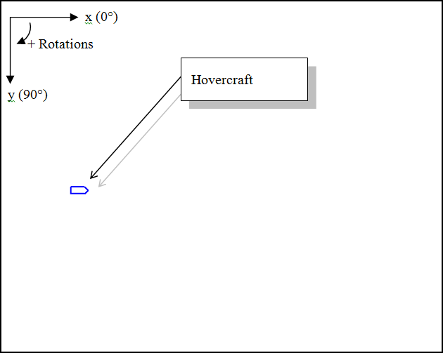
In this simulation, the world coordinate system has its x-axis pointing to the right, its y-axis pointing down toward the bottom of the screen, and the z-axis pointing into the screen. Even though this is a 2D example where all motion is confined to the x-y plane, you still need a z-axis about which the hovercraft will rotate. Also, the local, or body-fixed, coordinate system has its x-axis pointing toward the front of the hovercraft, its y-axis pointing to the starboard side, and its z-axis into the screen. The local coordinate system is fixed to the rigid body at its center of gravity location.
Model
The hovercraft modeled in this simulation is a simplified version of the hovercraft we’ll model in Chapter 17. You can refer to Chapter 17 for more details on that model. For convenience we repeat some of the basic properties of the model here. Figure 9-2 illustrates the main features of the model.
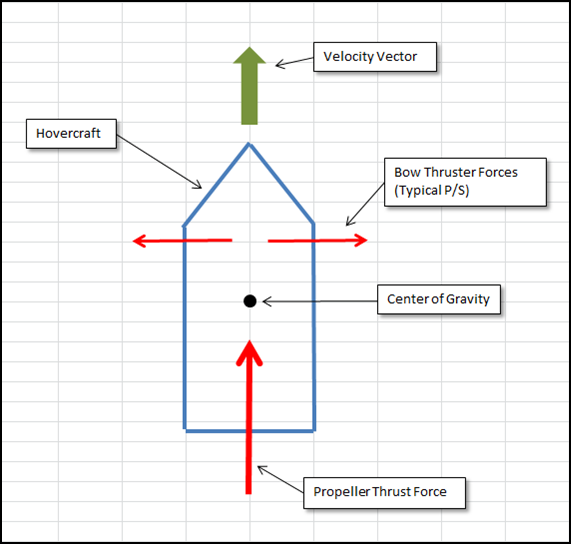
We’re assuming this hovercraft operates over smooth land and is fitted with a single airscrew propeller, located toward the aft end of the craft, that provides forward thrust. For controllability, the craft is fitted with two bow thrusters, one to port and the other to starboard. These bow thrusters are used to steer the hovercraft.
We use a simplified drag model where the only drag component is due to aerodynamic drag on the entire craft with a constant projected area. This model is similar to the one used in Chapter 8 for particle drag. A more rigorous model would consider the actual projected area of the craft as a function of the direction of relative velocity, as in the flight simulator example discussed in Chapter 15, as well as the frictional drag between the bottom of the craft’s skirt and the ground. We also assume that the center of drag—the point through which we can assume the drag force vector is applied—is located some distance aft of the center of gravity so as to give a little directional stability (that is, to counteract rotation). This serves the same function as the vertical tail fins on aircraft. Again, a more rigorous model would include the effects of rotation on aerodynamic drag, but we ignore that here.
In code, the first thing you need to do to represent this vehicle is
define a rigid-body class that contains all of the information you’ll need
to track it and calculate the forces and moments acting on it. This
RigidBody2D class is very similar to
the Particle class from Chapter 8, but with some additions mostly dealing with
rotation. Here’s how we did it:
class RigidBody2D {
public:
    float    fMass;       // total mass (constant)
    float    fInertia;    // mass moment of inertia
    float    fInertiaInverse;   // inverse of mass moment of inertia
    Vector    vPosition;        // position in earth coordinates
    Vector    vVelocity;        // velocity in earth coordinates
    Vector    vVelocityBody;    // velocity in body coordinates
    Vector    vAngularVelocity; // angular velocity in body coordinates

    float    fSpeed;            // speed
    float    fOrientation;      // orientation

    Vector    vForces;          // total force on body
    Vector    vMoment;          // total moment on body

    float    ThrustForce;       // Magnitude of the thrust force
    Vector    PThrust, SThrust; // bow thruster forces

    float    fWidth;            // bounding dimensions
    float    fLength;
    float    fHeight;

    Vector    CD; // location of center of drag in body coordinates
    Vector    CT; // location of center of propeller thrust in body coords.
    Vector    CPT; // location of port bow thruster thrust in body coords.
    Vector    CST; // location of starboard bow thruster thrust in body
                   // coords.

    float    ProjectedArea;     // projected area of the body

    RigidBody2D(void);
    void    CalcLoads(void);
    void    UpdateBodyEuler(double dt);
    void    SetThrusters(bool p, bool s);
    void    ModulateThrust(bool up);
};
The code comments briefly explain each property, and so far you’ve
seen all these properties somewhere in this book, so we won’t explain them
again here. That said, notice that several of these properties are the
same as those shown in the Particle
class from Chapter 8. These properties include fMass, vPosition, vVelocity, fSpeed, vForces, and fRadius. All of the other properties are new and
required to handle the rotational motion aspects of rigid bodies.
The RigidBody2D constructor is
straightforward, as shown next, and simply initializes all the properties
to some arbitrarily tuned values we decided worked well. In Chapter 17, you’ll see how we model a more realistic
hovercraft.
RigidBody2D::RigidBody2D(void)
{
    fMass = 100;
    fInertia = 500;
    fInertiaInverse = 1/fInertia;
    vPosition.x = 0;
    vPosition.y = 0;
    fWidth = 10;
    fLength = 20;
    fHeight = 5;
    fOrientation = 0;

    CD.x = −0.25*fLength;
    CD.y = 0.0f;
    CD.z = 0.0f;

    CT.x = −0.5*fLength;
    CT.y = 0.0f;
    CT.z = 0.0f;

    CPT.x = 0.5*fLength;
    CPT.y = −0.5*fWidth;
    CPT.z = 0.0f;

    CST.x = 0.5*fLength;
    CST.y = 0.5*fWidth;
    CST.z = 0.0f;

    ProjectedArea = (fLength + fWidth)/2 * fHeight; // an approximation
    ThrustForce = _THRUSTFORCE;
}
As in the particle simulator of Chapter 8, you’ll
notice here that the Vector class is
actually a triple (that is, it has three
components—x, y, and z). Since this is a 2D example, the
z components will always be 0, except in the case of
the angular velocity vector where only the z
component will be used (since rotation occurs only about the z-axis). The
class that we use in this example is discussed in Appendix A. The reason we didn’t write a separate 2D
vector class, one with only x and
y components, is because we’ll extend this code to 3D
later and wanted to get you accustomed to using the 3D vector class.
Besides, it’s pretty easy to create a 2D vector class from the 3D class by
simply stripping out the z component.
As with the particle example of Chapter 8, we
need a CalcLoads method for the rigid
body. As before, this method will compute all the loads acting on the
rigid body, but now these loads include both forces and moments that will
cause rotation. CalcLoads looks like
this:
void    RigidBody2D::CalcLoads(void)
{
    Vector    Fb;        // stores the sum of forces
    Vector    Mb;        // stores the sum of moments
    Vector    Thrust;    // thrust vector

    // reset forces and moments:
    vForces.x = 0.0f;
    vForces.y = 0.0f;
    vForces.z = 0.0f;    // always zero in 2D

    vMoment.x = 0.0f;    // always zero in 2D
    vMoment.y = 0.0f;    // always zero in 2D
    vMoment.z = 0.0f;

    Fb.x = 0.0f;
    Fb.y = 0.0f;
    Fb.z = 0.0f;

    Mb.x = 0.0f;
    Mb.y = 0.0f;
    Mb.z = 0.0f;

    // Define the thrust vector, which acts through the craft's CG
    Thrust.x = 1.0f;
    Thrust.y = 0.0f;
    Thrust.z = 0.0f;     // zero in 2D
    Thrust *= ThrustForce;

    // Calculate forces and moments in body space:
    Vector   vLocalVelocity;
    float    fLocalSpeed;
    Vector   vDragVector;
    float    tmp;
    Vector   vResultant;
    Vector   vtmp;

    // Calculate the aerodynamic drag force:
        // Calculate local velocity:
        // The local velocity includes the velocity due to
        // linear motion of the craft,
        // plus the velocity at each element
        // due to the rotation of the craft.

        vtmp = vAngularVelocity^CD; // rotational part
        vLocalVelocity = vVelocityBody + vtmp;

        // Calculate local air speed
        fLocalSpeed = vLocalVelocity.Magnitude();

        // Find the direction in which drag will act.
        // Drag always acts in line with the relative
        // velocity but in the opposing direction
        if(fLocalSpeed > tol)
        {
            vLocalVelocity.Normalize();
            vDragVector = -vLocalVelocity;

            // Determine the resultant force on the element.
            tmp = 0.5f * rho * fLocalSpeed*fLocalSpeed
                         * ProjectedArea;
            vResultant = vDragVector * _LINEARDRAGCOEFFICIENT * tmp;

            // Keep a running total of these resultant forces
            Fb += vResultant;

            // Calculate the moment about the CG
            // and keep a running total of these moments

            vtmp = CD^vResultant;
            Mb += vtmp;
        }

        // Calculate the Port & Starboard bow thruster forces:
        // Keep a running total of these resultant forces

        Fb += PThrust;


        // Calculate the moment about the CG of this element's force
        // and keep a running total of these moments (total moment)
        vtmp = CPT^PThrust;
        Mb += vtmp;

        // Keep a running total of these resultant forces (total force)
        Fb += SThrust;

        // Calculate the moment about the CG of this element's force
        // and keep a running total of these moments (total moment)
        vtmp = CST^SThrust;
        Mb += vtmp;

    // Now add the propulsion thrust
    Fb += Thrust; // no moment since line of action is through CG

    // Convert forces from model space to earth space
    vForces = VRotate2D(fOrientation, Fb);

    vMoment += Mb;
}
The first thing that CalcLoads
does is initialize the force and moment variables that will contain the
total of all forces and moments acting on the craft at any instant in
time. Just as we must aggregate forces, we must also aggregate moments.
The forces will be used along with the linear equation of motion to
compute the linear displacement of the rigid body, while the moments will
be used with the angular equation of motion to compute the orientation of the body.
The function then goes on to define a vector representing the
propeller thrust, Thrust. The propeller
thrust vector acts in the positive (local) x-direction and has a magnitude
defined by ThrustForce, which the user
sets via the keyboard interface (we’ll get to that later). Note that if
ThrustForce is negative, then the
thrust will actually be a reversing thrust instead of a forward
thrust.
After defining the thrust vector, this function goes on to calculate
the aerodynamic drag acting on the hovercraft. These calculations are very
similar to those discussed in Chapter 17. The
first thing to do is determine the relative velocity at the center of
drag, considering both linear and angular motion. You’ll need the
magnitude of the relative velocity vector when calculating the magnitude
of the drag force, and you’ll need the direction of the relative velocity
vector to determine the direction of the drag force since it always
opposes the velocity vector. The line vtmp =
vAngularVelocity^CD computes the linear velocity at the drag
center by taking the vector cross product of the angular velocity vector
with the position vector of the drag center, CD. The result is stored in a temporary vector,
vtmp, and then added vectorially to the
body velocity vector, vVelocityBody.
The result of this vector addition is a velocity vector representing the
velocity of the point defined by CD,
including contributions from the body’s linear and angular motion. We
compute the actual drag force, which acts in line with but in a direction
opposing the velocity vector, in a manner similar to that for particles,
using a simple formula relating the drag force to the speed squared,
density of air, projected area, and a drag coefficient. The following code
performs this calculation:
            vLocalVelocity.Normalize();
            vDragVector = -vLocalVelocity;

            // Determine the resultant force on the element.
            tmp = 0.5f * rho * fLocalSpeed*fLocalSpeed
                         * ProjectedArea;
            vResultant = vDragVector * _LINEARDRAGCOEFFICIENT * tmp;
Note that the drag coefficient, LINEARDRAGCOEFFICIENT, is defined as
follows:
#define LINEARDRAGCOEFFICIENT 1.25f
Once the drag force is determined, it gets aggregated in the total force vector as follows:
Fb += vResultant;
In addition to aggregating this force, we must aggregate the moment due to that force in the total moment vector as follows:
              vtmp = CD^vResultant;
              Mb += vtmp;
The first line computes the moment due to the drag force by taking the vector cross product of the position vector, to the center of drag, with the drag force vector. The second line adds this force to the variable, accumulating these moments.
With the drag calculation complete, CalcLoads proceeds to calculate the forces and
moments due to the bow thrusters, which may be active or inactive at any
given time.
        Fb += PThrust;

        vtmp = CPT^PThrust;
        Mb += vtmp;
The first line aggregates the port bow thruster force into Fb. PThrust
is a force vector computed in the SetThrusters method in response to your keyboard
input. The next two lines compute and aggregate the moment due to the
thruster force. A similar set of code lines follows, computing the force
and moment due to the starboard bow thruster.
Next, the propeller thrust force is added to the running total of forces. Remember, since the propeller thrust force acts through the center of gravity, there is no moment to worry about. Thus, all we need is:
Fb += Thrust; // no moment since line of action is through CG
Finally, the total force is transformed from local coordinates to world coordinates via a vector rotation given the orientation of the hovercraft, and the total forces and moments are stored so they are available when it comes time to integrate the equations of motion at each time step.
As you can see, computing loads on a rigid body is a bit more
complex than what you saw earlier when dealing with particles. This, of
course, is due to the nature of rigid bodies being able to rotate. What’s
nice, though, is that all this new complexity is encapsulated in CalcLoads, and the rest of the simulator is
pretty much the same as when we’re dealing with particles.
Transforming Coordinates
Let’s talk about transformation from local to world coordinates a bit more
since you’ll see this sort of transform again in a few places. When
computing forces acting on the rigid body, we want those forces in a
vector form relative to the coordinates that are fixed with respect to
the hovercraft (e.g., relative to the body’s center of gravity with the
x-axis pointing toward the front of the body and the y-axis pointing
toward the starboard side). This simplifies our calculations of forces
and moments. However, when integrating the equation of motion to see how
the body translates in world coordinates, we use the equations of motion in world coordinates, requiring us to
represent the aggregate force in world coordinates. That’s why we
rotated the aggregate force at the end of the CalcLoads method.
In two dimensions, the coordinate transformation involves a little
trigonometry as shown in the following VRotate2D function:
Vector    VRotate2D( float angle, Vector u)
{
    float    x,y;

    x = u.x * cos(DegreesToRadians(-angle)) +
        u.y * sin(DegreesToRadians(-angle));
    y = -u.x * sin(DegreesToRadians(-angle)) +
        u.y * cos(DegreesToRadians(-angle));

    return Vector( x, y, 0);
}
The angle here represents the orientation of the local, body fixed
coordinate system with respect to the world coordinate system. When
converting from local coordinates to world coordinates, use a positive
angle; use a negative angle when going the other way. This is just the
convention we’ve adopted so transformations from local coordinates to
world coordinates are positive. You can see we actually take the
negative of the angle parameter, so
in reality you could do away with that negative, and then
transformations from local coordinates to world coordinates would
actually be negative. It’s your preference. You’ll see this function
used a few more times in different situations before the end of this
chapter.
Integrator
The UpdateBodyEuler method
actually integrates the equations of motion for the rigid
body. Since we’re dealing with a rigid body, unlike a particle, we have
two equations of motion: one for translation, and the other for
rotation. The following code sample shows UpdateBodyEuler.
void    RigidBody2D::UpdateBodyEuler(double dt)
{
        Vector a;
        Vector dv;
        Vector ds;
        float  aa;
        float  dav;
        float  dr;

        // Calculate forces and moments:
        CalcLoads();

        // Integrate linear equation of motion:
        a = vForces / fMass;

        dv = a * dt;
        vVelocity += dv;

        ds = vVelocity * dt;
        vPosition += ds;

        // Integrate angular equation of motion:
        aa = vMoment.z / fInertia;

        dav = aa * dt;

        vAngularVelocity.z += dav;

        dr = RadiansToDegrees(vAngularVelocity.z * dt);
        fOrientation += dr;

        // Misc. calculations:
        fSpeed = vVelocity.Magnitude();
        vVelocityBody = VRotate2D(-fOrientation, vVelocity);
}
As the name of this method implies, we’ve implemented Euler’s
method of integration as described in Chapter 7. Integrating the linear equation of
motion for a rigid body follows exactly the same steps we used for
integrating the linear equation of motion for particles. All that’s
required is to divide the aggregate forces acting on a body by the mass
of the body to get the body’s acceleration. The line of code a = vForces / fMass does just this. Notice
here that a is a Vector, as is vForces. fMass is a scalar, and the / operator defined in the Vector class takes care of dividing each
component of the vForces vector by
fMass and setting the corresponding
components in a. The change in
velocity, dv, is equal to
acceleration times the change in time, dt. The body’s new velocity is then computed
by the line vVelocity += dv. Here
again, vVelocity and dv are Vectors and the += operator takes care of the vector
arithmetic. This is the first actual integration for translation.
The second integration takes place in the next few lines, where we
determine the body’s displacement and new position by integrating its
velocity. The line ds = vVelocity *
dt determines the displacement, or change in the body’s
position, and the line vPosition +=
ds computes the new position by adding the displacement to the
body’s old position. That’s it for translation.
The next order of business is to integrate the angular equation of
motion to find the body’s new orientation. The line aa =
vMoment.z / fInertia; computes the body’s angular acceleration
by dividing the aggregate moment acting on the body by its mass moment
of inertia. aa is a scalar, as is
fInertia since this is a 2D problem.
In 3D, things are a bit more complicated, and we’ll get to that in Chapter 11.
We compute the change in angular velocity, dav, a scalar, by multiplying aa by the time step size, dt. The new angular velocity is simply the old
velocity plus the change: vAngularVelocity.z +=
dav. The change in orientation is equal to the new angular
velocity multiplied by the time step: vAngularVelocity.z * dt. Notice that we
convert the change in orientation from radians to degrees here since
we’re keeping track of orientation in degrees. You don’t really have to,
so long as you’re consistent.
The last line in UpdateBodyEuler computes the body’s linear
speed by transforming the magnitude of its velocity vector to local,
body coordinates. Recall in CalcLoads
that we require the body’s velocity in body-fixed coordinates in order
to compute the drag force on the body.
Rendering
In this simple example, rendering the virtual hovercraft is just a little more involved than rendering the particles in the example from Chapter 8. All we do is draw a few connected lines using Windows API calls wrapped in our own functions to hide some of the Windows-specific code. The following code snippet is all we need to render the hovercraft:
void    DrawCraft(RigidBody2D    craft, COLORREF clr)
{
    Vector    vList[5];
    double    wd, lg;
    int       i;
    Vector    v1;

    wd = craft.fWidth;
    lg = craft.fLength;
    vList[0].x = lg/2;     vList[0].y = wd/2;
    vList[1].x = -lg/2;    vList[1].y = wd/2;
    vList[2].x = -lg/2;    vList[2].y = -wd/2;
    vList[3].x = lg/2;     vList[3].y = -wd/2;
    vList[4].x = lg/2*1.5; vList[4].y = 0;
    for(i=0; i<5; i++)
    {
        v1 = VRotate2D(craft.fOrientation, vList[i]);
        vList[i] = v1 + craft.vPosition;
    }

    DrawLine(vList[0].x, vList[0].y, vList[1].x, vList[1].y, 2, clr);
    DrawLine(vList[1].x, vList[1].y, vList[2].x, vList[2].y, 2, clr);
    DrawLine(vList[2].x, vList[2].y, vList[3].x, vList[3].y, 2, clr);
    DrawLine(vList[3].x, vList[3].y, vList[4].x, vList[4].y, 2, clr);
    DrawLine(vList[4].x, vList[4].y, vList[0].x, vList[0].y, 2, clr);
}
You can use your own rendering code here, of course, and all you
really need to pay close attention to is transforming the coordinates
for the outline of the hovercraft from body to world coordinates. This
involves rotating the vertex coordinates from body-fixed space using the
VRotate2D function and then adding
the position of the center of gravity of the hovercraft to each
transformed vertex. These lines take care of this coordinate
transformation:
    for(i=0; i<5; i++)
    {
        v1 = VRotate2D(craft.fOrientation, vList[i]);
        vList[i] = v1 + craft.vPosition;
    }
The Basic Simulator
The heart of this simulation is handled by the RigidBody2D class described earlier. However, we
need to show you how that class is used in the context of the main
program. This simulator is very similar to that shown in Chapter 8 for particles, so if you’ve read that chapter
already you can breeze through this section.
First, we define a few global variables as follows:
// Global Variables:
int            FrameCounter = 0;
RigidBody2D    Craft;
FrameCounter counts the number of
time steps integrated before the graphics display is updated. How many
time steps you allow the simulation to integrate before updating the
display is a matter of tuning. You’ll see how this is used momentarily
when we discuss the UpdateSimulation
function. Craft is a RigidBody2D type that will represent our virtual
hovercraft.
For the most part, Craft is
initialized in accordance with the RigidBody2D constructor shown earlier. However,
its position is at the origin, so we make a call to the following Initialize function to locate the Craft in the middle of the screen vertically and
on the left side. We set its orientation to 0 degrees so it points toward
the right side of the screen:
bool    Initialize(void)
{
    Craft.vPosition.x = _WINWIDTH/10;
    Craft.vPosition.y = _WINHEIGHT/2;
    Craft.fOrientation = 0;

    return true;
}
OK, now let’s consider UpdateSimulation as shown in the code snippet
below. This function gets called every cycle through the program’s main
message loop and is responsible for making appropriate function calls to
update the hovercraft’s position and orientation, as well as rendering the
scene. It also checks the states of the keyboard arrow keys and makes
appropriate function calls:
void    UpdateSimulation(void)
{
    double  dt = _TIMESTEP;
    RECT    r;

    Craft.SetThrusters(false, false);

    if (IsKeyDown(VK_UP))
        Craft.ModulateThrust(true);

    if (IsKeyDown(VK_DOWN))
        Craft.ModulateThrust(false);

    if (IsKeyDown(VK_RIGHT))
        Craft.SetThrusters(true, false);

    if (IsKeyDown(VK_LEFT))
        Craft.SetThrusters(false, true);

    // update the simulation
    Craft.UpdateBodyEuler(dt);

    if(FrameCounter >= _RENDER_FRAME_COUNT)
    {
        // update the display
        ClearBackBuffer();

        DrawCraft(Craft, RGB(0,0,255));

        CopyBackBufferToWindow();
        FrameCounter = 0;
    } else
        FrameCounter++;

    if(Craft.vPosition.x > _WINWIDTH) Craft.vPosition.x = 0;
    if(Craft.vPosition.x < 0) Craft.vPosition.x = _WINWIDTH;
    if(Craft.vPosition.y > _WINHEIGHT) Craft.vPosition.y = 0;
    if(Craft.vPosition.y < 0) Craft.vPosition.y = _WINHEIGHT;
}
The local variable dt represents
the small yet finite amount of time, in seconds, over which each
integration step is taken. The global define
_TIMESTEP stores the time step, which we have set to 0.001
seconds. This value is subject to tuning.
The first action UpdateSimulation
takes is to reset the states of the bow thrusters to inactive by calling
the SetThrusters method as
follows:
Craft.SetThrusters(false, false);
Next, the keyboard is polled using the function IsKeyDown. This is a wrapper function we created
to encapsulate the necessary Windows API calls used to check key states.
If the up arrow key is pressed, then the RigidBody2D method ModulateThrust is called, as shown here:
Craft.ModulateThrust(true);
If the down arrow key is pressed, then ModulateThrust is called, passing false instead of true.
ModulateThrust looks like
this:
void    RigidBody2D::ModulateThrust(bool up)
{
    double    dT = up ? _DTHRUST:-_DTHRUST;

    ThrustForce += dT;

    if(ThrustForce > _MAXTHRUST) ThrustForce = _MAXTHRUST;
    if(ThrustForce < _MINTHRUST) ThrustForce = _MINTHRUST;
}
All it does is increment the propeller thrust force by a small
amount, either increasing it or decreasing it, depending on the value of
the up parameter.
Getting back to UpdateSimulation,
we make a couple more calls to IsKeyDown, checking the states of the left and
right arrow keys. If the left arrow key is down, then the RigidBody2D method SetThrusters is called, passing false as the first parameter and true as the second parameter. If the right arrow
key is down, these parameter values are reversed. SetThrusters looks like this:
void    RigidBody2D::SetThrusters(bool p, bool s)
{
    PThrust.x = 0;
    PThrust.y = 0;
    SThrust.x = 0;
    SThrust.y = 0;

    if(p)
        PThrust.y = _STEERINGFORCE;
    if(s)
        SThrust.y = -_STEERINGFORCE;
}
It resets the port and starboard bow thruster thrust vectors and
then sets them according to the parameters passed in SetThrusters. If p is true,
then a right turn is desired and a port thrust force, PThrust, is created, pointing toward the
starboard side. This seems opposite of what you’d expect, but it is the
port bow thruster that is fired, pushing the bow of the hovercraft toward
the right (starboard) side. Similarly, if s is true, a
thrust force is created that will push the bow of the hovercraft to the
left (port) side.
Now with the thrust forces managed, UpdateSimulation makes the call:
Craft.UpdateBodyEuler(dt)
UpdateBodyEuler integrates the
equations of motion as discussed earlier.
The next segment of code checks the value of the frame counter. If
the frame counter has reached the defined number of frames (stored in
_RENDER_FRAME_COUNT), then the back
buffer is cleared to prepare it for drawing upon and ultimately copying to
the screen.
Finally, the last four lines of code wrap the hovercraft’s position around the edges of the screen.
Tuning
You’ll probably want to tune this example to run well on your computer since we didn’t implement any profiling for processor speed. Moreover, you should tune the various parameters governing the behavior of the hovercraft to see how it responds. The way we have it set up now makes the hovercraft exhibit a soft sort of response to turning—that is, upon application of turning forces, the craft will tend to keep tracking in its original heading for a bit even while yawed. It will not respond like a car would turn. You can change this behavior, of course.
Some things we suggest you play with include the time step size and the various constants we’ve defined as follows:
#define  _THRUSTFORCE      5.0f
#define  _MAXTHRUST        10.0f
#define  _MINTHRUST        0.0f
#define  _DTHRUST          0.001f
#define  _STEERINGFORCE    3.0f
#define  _LINEARDRAGCOEFFICIENT    1.25f
_THRUSTFORCE is the initial
magnitude of the propeller thrust force. _MAXTHRUST and _MINTHRUST set upper and lower bounds to this
force, which is modulated by the user pressing the up and down arrow keys.
_DTHRUST is the incremental change in
thrust in response to the user pressing the up and down arrow keys.
_STEERINGFORCE is the magnitude of the
bow thruster forces. You should definitely play with this value to see how
the behavior of the hovercraft changes. Finally, _LINEARDRAGCOEFFICIENT is the drag coefficient
used to compute aerodynamic drag. This is another good value to play with
to see how behavior is affected. Speaking of drag, the location of the
center of drag that’s initialized in the RigidBody2D constructor is a good parameter to
change in order to understand how it affects the behavior of the
hovercraft. It influences the craft’s directional stability, which affects
its turning radius—particularly at higher speeds.