
Chapter 7. Real-Time Simulations
This chapter is the first in a series of chapters designed to give you a thorough introduction to the subject of real-time simulation. We say introduction because the subject is too vast and complex to adequately treat in a few chapters; however, we say thorough because we’ll do more than touch on real-time simulations. In fact, we’ll walk you through the development of two simple simulations, one in two dimensions and the other in three dimensions.
What we hope to do is give you enough of an understanding of this subject so that you can pursue it further with confidence. In other words, we want you to have a solid understanding of the fundamentals before jumping in to use someone else’s physics engine, or venturing out to write your own.
In the context of this book, a real-time simulation is a process
whereby you calculate the state of the object (or objects) you’re trying to
represent on the fly. You don’t rely on prescripted motion sequences to
animate your object, but instead you rely on your physics model, the
equations of motion, and your differential equation solver to take care of
the motion of your object as the simulation progresses. This sort of
simulation can be used to model rigid bodies like the airplane in our
FlightSim example, or flexible bodies
such as cloth and human figures. Perhaps one of the most fundamental aspects
of implementing a real-time rigid-body simulator is solving the equations of
motion using numerical integration techniques. For this reason, we’ll spend
this entire chapter explaining the numerical integration techniques that
you’ll use later in the 2D and 3D simulators that we’ll develop.
If you refer back for a moment to Chapter 4, where we outlined a generic procedure for solving kinetics problems, you’ll see that we’ve covered a lot of ground so far. The preceding chapters have shown you how to estimate mass properties and develop the governing equations of motion. This chapter will show you how to solve the equations of motion in order to determine acceleration, velocity, and displacement. We’ll follow this chapter up with several showing you how to implement both 2D and 3D rigid-body simulations.
Integrating the Equations of Motion
By now you should have a thorough understanding of the dynamic equations of motion for particles and rigid bodies. If not, you may want to go back and review Chapter 1 through Chapter 4 before reading this one. The next aspect of dealing with the equations of motion is actually solving them in your simulation. The equations of motion that we’ve been discussing can be classified as ordinary differential equations. In Chapter 2 and Chapter 4, you were able to solve these differential equations explicitly since you were dealing with simple functions for acceleration, velocity, and displacement. This won’t be the case for your simulations. As you’ll see in later chapters, force and moment calculations for your system can get pretty complicated and may even rely on tabulated empirical data, which will prevent you from writing simple mathematical functions that can be easily integrated. This means that you have to use numerical integration techniques to approximately integrate the equations of motion. We say approximately because solutions based on numerical integration won’t be exact and will have a certain amount of error depending on the chosen method.
We’re going to start with a rather informal explanation of how we’ll apply numerical integration because it will be easier to grasp. Later we’ll get into some of the formal mathematics. Take a look at the differential equation of linear motion for a particle (or rigid body’s center of mass):
| F = m dv/dt |
Recall that this equation is a statement of force equals mass times acceleration, where F is force, m is mass, and dv/dt is the time derivative of velocity, which is acceleration. In the simple examples of the earlier chapters of this book, we rewrote this equation in the following form so it could be integrated explicitly:
| dv/dt = F/m |
| dv = (F/m) dt |
One way to interpret this equation is that an infinitesimally small change in velocity, dv, is equal to (F/m) times an infinitesimally small change in time. In earlier examples, we integrated explicitly by taking the definite integral of the left side of this equation with respect to velocity and the right side with respect to time. In numerical integration you have to take finite steps in time, thus dt goes from being infinitely small to some discrete time increment, ∆t, and you end up with a discrete change in velocity, ∆v:
| ∆v = (F/m) ∆t |
It is important to notice here that this does not give a formula for instantaneous velocity; instead, it gives you only an approximation of the change in velocity. Thus, to approximate the actual velocity of your particle (or rigid body), you have to know what its velocity was before the time change ∆t. At the start of your simulation, at time 0, you have to know the starting velocity of your particle. This is an initial condition and is required in order to uniquely define your particle’s velocity as you step through time using this equation:[17]
| vt+∆t = vt + (F/m) ∆t |
where the initial condition is:
| vt=0 = v0 |
Here vt is velocity at some time t, vt+∆t is velocity at some time plus the time step, ∆t is the time step, and v0 is the initial velocity at time 0.
You can integrate the linear equation of motion one more time in order to approximate your particle’s displacement (or position). Once you’ve determined the new velocity value, at time t + ∆t, you can approximate displacement using:
| st+∆t = st + ∆t (vt+∆t) |
where the initial condition on displacement is:
| st=0 = s0 |
The integration technique discussed here is known as Euler’s method, and it is the most basic integration method. While Euler’s method is easy to grasp and fairly straightforward to implement, it isn’t necessarily the most accurate method.
You can reason that the smaller you make your time step—that is, as ∆t approaches dt—the closer you’ll get to the exact solution. There are, however, computational problems associated with using very small time steps. Specifically, you’ll need a huge number of calculations at very small ∆t’s, and since your calculations won’t be exact (depending on numerical precision you’ll be rounding off and truncating numbers), you’ll end up with a buildup of round-off error. This means that there is a practical limit as to how small a time step you can take. Fortunately, there are several numerical integration techniques at your disposal that are designed to increase accuracy for reasonable step sizes.
Even though we used the linear equation of motion for a particle, this integration technique (and the ones we’ll show you later) applies equally well to the angular equations of motion.
Euler’s Method
The preceding explanation of Euler’s method was, as we said, informal. To treat Euler’s method in a more mathematically rigorous way, we’ll look at the Taylor series expansion of a general function, y(x). Taylor’s theorem lets you approximate the value of a function at some point by knowing something about that function and its derivatives at some other point. This approximation is expressed as an infinite polynomial series of the form:
| y(x + ∆x) = y(x) + (∆x) y'(x) + ((∆x)2 / 2!) y''(x) + ((∆x)3 / 3!) y'''(x) + · · · |
where y is some function of x, (x + ∆x) is the new value of x at which you want to approximate y, y' is the first derivative of y, y'' is the second derivative of y, and so on.
In the case of the equation of motion discussed in the preceding section, the function that you are trying to approximate is the velocity as a function of time. Thus, you can write v(t) instead of y(x), which yields the Taylor expansion:
| v(t + ∆t) = v(t) + (∆t) v'(t) + ((∆t)2 / 2!) v''(t) + ((∆t)3 / 3!) v'''(t) + · · · |
Note here that v'(t) is equal to dv/dt, which equals F/m in the example equation of motion discussed in the preceding section. Note also that you know the value of v at time t. What you want to find is the value of v at time t + ∆t knowing v at time t and its derivative at time t. As a first approximation, and since you don’t know anything about v’s second, third, or higher derivatives, you can truncate the polynomial series after the term (∆t) v'(t), which yields:
| v(t + ∆t) = v(t) + (∆t) v'(t) |
This is the Euler integration formula that you saw in the last section. Since Euler’s formula goes out only to the term that includes the first derivative, the rest of the series that was left off is the truncation error. These terms that were left off are called higher-order terms, and getting rid of them results in a first-order approximation. The rationale behind this approximation is that the further you go in the series, the smaller the terms and the less influence they have on the approximation. Since ∆t is presumed to be a small number, ∆t2 is even smaller, ∆t3 even smaller, and so on, and since these ∆t terms appear in the numerators, each successively higher-order term gets smaller and smaller. In this case, the first truncated term, ((∆t)2 / 2!) v''(t), dominates the truncation error, and this method is said to have an error of order (∆t)2.
Geometrically, Euler’s method approximates a new value, at the current step, for the function under consideration by extrapolating in the direction of the derivative of the function at the previous step. This is illustrated in Figure 7-1.
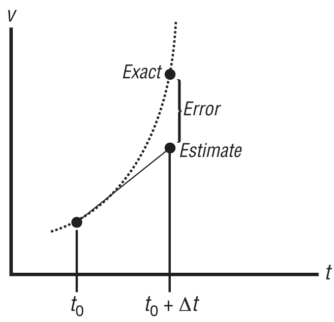
Figure 7-1 illustrates the truncation error and shows that Euler’s method will result in a polygonal approximation of the smooth function under consideration. Clearly, if you decrease the step size, you increase the number of polygonal segments and better approximate the function. As we said before, though, this isn’t always efficient to do since the number of computations in your simulation will increase and round-off error will accumulate more rapidly.
To illustrate Euler’s method in practice, let’s examine the linear equation of motion for the ship example of Chapter 4:
| T – (C v) = ma |
where T is the propeller’s thrust, C is a drag coefficient, v is the ship’s velocity, m its mass, and a its acceleration.
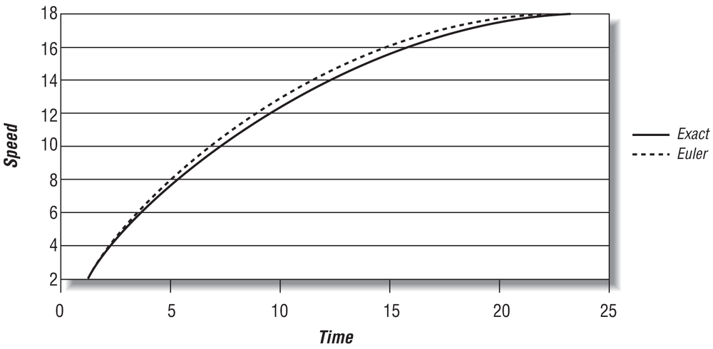
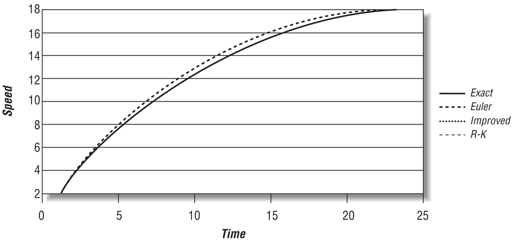
Figure 7-2 shows the Euler integration solution, using a 0.5s time step, superimposed over the exact solution derived in Chapter 4 for the ship’s speed over time.
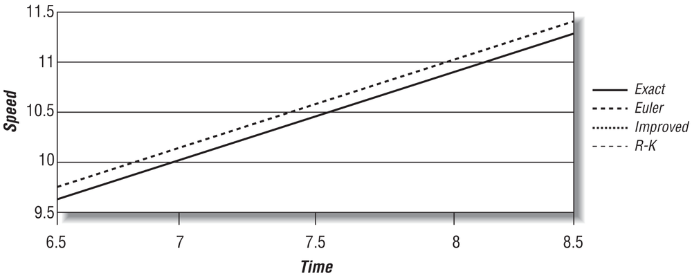
Zooming in on this graph allows you to see the error in the Euler approximation. This is shown in Figure 7-3.
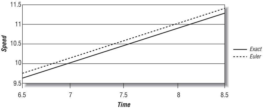
Table 7-1 shows the numerical values of speed versus time for the range shown in Figure 7-3. Also shown in Table 7-1 is the percent difference, the error, between the exact solution and the Euler solution at each time step.
Time (s) | Velocity, exact (m/s) | Velocity, Euler (m/s) | Error |
6.5 | 9.559084 | 9.733158 | 1.82% |
7 | 10.06829 | 10.2465 | 1.77% |
7.5 | 10.55267 | 10.73418 | 1.72% |
8 | 11.01342 | 11.19747 | 1.67% |
8.5 | 11.4517 | 11.63759 | 1.62% |
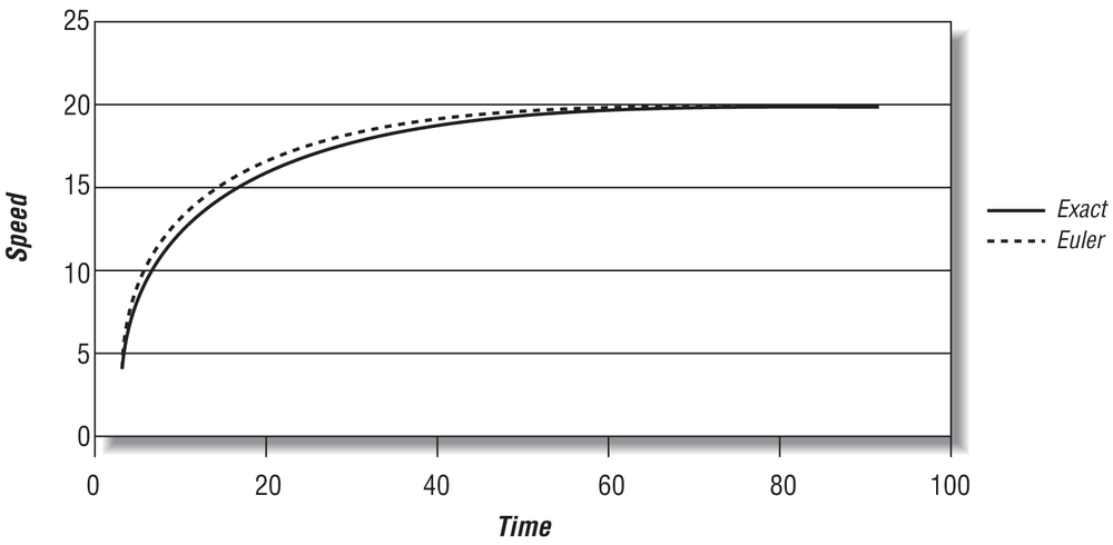
As you can see, the truncation error in this example isn’t too bad. It could be better, though, and we’ll show you some more accurate methods in a moment. Before that, however, you should notice that in this example Euler’s method is also stable—that is, it converges well with the exact solution as shown in Figure 7-4, where we’ve carried the time range out further.
Here’s a code snippet that implements Euler’s method for this example:
// Global Variables
float     T;     // thrust
float     C;     // drag coefficient
float     V;     // velocity
float     M;     // mass
float     S;     // displacement

.
.
.

// This function progresses the simulation by dt seconds using
// Euler's basic method
void StepSimulation(float dt)
{
     float     F;     // total force
     float     A;     // acceleration
     float     Vnew;  // new velocity at time t + dt
     float     Snew;  // new position at time t + dt

     // Calculate the total force
     F = (T − (C * V));

     // Calculate the acceleration
     A = F / M;

     // Calculate the new velocity at time t + dt
     // where V is the velocity at time t
     Vnew = V + A * dt;

     // Calculate the new displacement at time t + dt
     // where S is the displacement at time t
     Snew = S + Vnew * dt;

     // Update old velocity and displacement with the new ones
     V = Vnew;
     S = Snew;
}
Although Euler’s method is stable in this example, that isn’t always so, depending on the problem you’re trying to solve. This is something that you must keep in mind when implementing any numerical integration scheme. What we mean by stable here is that, in this case, the Euler solution converges with the exact solution. An unstable solution could manifest errors in two ways. First, successive values could oscillate above and below the exact solution, never quite converging on it. Second, successive values could diverge from the exact solution, creating a greater and greater error over time.
Take a look at Figure 7-5. This figure shows how Euler’s method can become very unstable. What you see in the graph represents the vibratory motion of a spring-mass system. This is a simple dynamical system that should exhibit regular sinusoidal motion.
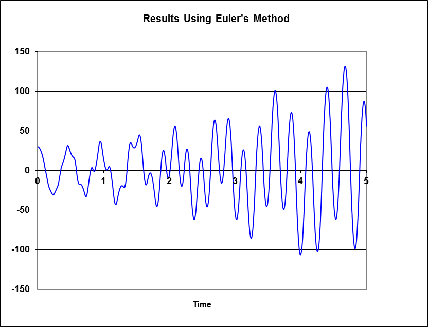
It’s clear from the figure that using Euler’s method yields terribly unstable results. You can see how the motion amplitude continues to grow. If this were a game, say, where you have a few objects connected by springs interacting with one another, then this sort of instability would manifest itself by wildly unrealistic motion of those objects. Worse yet, the simulation could blow up, numerically speaking.
Often, your choice of step size affects stability where smaller step sizes tend to eliminate or minimize instability and larger steps aggravate the problem. If you’re working with a particularly unwieldy function, you might find that you have to decrease your step size substantially in order to achieve stability. This, however, increases the number of computations you need to make. One way around this difficulty is to employ what’s called an adaptive step size method, in which you change your step size on the fly depending on the magnitude of a predicted amount of truncation error from one step to the next. If the truncation error is too large, then you back up a step, decrease your step size, and try again.
One way to implement this for Euler’s method is to first take a step of size ∆t to obtain an estimate at time t + ∆t, and then take two steps (starting from time t again) of size ∆t/2 to obtain another estimate at time t + ∆t. Since we’ve been talking velocity in the examples so far, let’s call the first estimate v1 and the second estimate v2.[18] A measure of the truncation error is then:
| et = |v1 – v2| |
If you wish to keep the truncation error within a specified limit, eto, then you can use the following formula to find out what your step size should be in order to maintain the desired accuracy:
| ∆tnew = ∆told (eto / et) (1/2) |
Here, ∆told is the old time step and ∆tnew is the new one that you should use to maintain the desired accuracy. You’ll have to make this check for each time step, and if you find that the error warrants a smaller time step, then you’ll have to back up a step and repeat it with the new time step.
Here’s a revised StepSimulation
function that implements this adaptive step size technique, checking the
truncation error on the velocity integration:
// New global variable
float     eto;     // truncation error tolerance

// This function progresses the simulation by dt seconds using
// Euler's basic method with an adaptive step size
void StepSimulation(float dt)
{
     float     F;     // total force
     float     A;     // acceleration
     float     Vnew;  // new velocity at time t + dt
     float     Snew;  // new position at time t + dt
     float     V1, V2; // temporary velocity variables
     float     dtnew;  // new time step
     float     et;     // truncation error

     // Take one step of size dt to estimate the new velocity
     F = (T − (C * V));
     A = F / M;
     V1 = V + A * dt;

     // Take two steps of size dt/2 to estimate the new velocity
     F = (T − (C * V));
     A = F / M;
     V2 = V + A * (dt/2);

     F = (T − (C * V2));
     A = F / M;
     V2 = V2 + A * (dt/2);

     // Estimate the truncation error
     et = absf(V1 − V2);

     // Estimate a new step size
     dtnew = dt * SQRT(eto/et);


     if (dtnew < dt)
     { // take at step at the new smaller step size
          F = (T − (C * V));
          A = F / M;
          Vnew = V + A * dtnew;
          Snew = S + Vnew * dtnew;
     } else
     { // original step size is okay
          Vnew = V1;
          Snew = S + Vnew * dt;
     }

     // Update old velocity and displacement with the new ones
     V = Vnew;
     S = Snew;
}
Better Methods
At this point, you might be wondering why you can’t simply use more terms in the Taylor series to reduce the truncation error of Euler’s method. In fact, this is the basis for several integration methods that offer greater accuracy than Euler’s basic method for a given step size. Part of the difficulty associated with picking up more terms in the Taylor’s series expansion is in being able to determine the second, third, fourth, and higher derivatives of the function you’re trying to integrate. The way around this problem is to perform additional Taylor series expansions to approximate the derivatives of the function under consideration and then substitute those values back into your original expansion.
Taking this approach to include one more Taylor term beyond the basic Euler method yields a so-called improved Euler method that has a reduced truncation error on the order of (∆t)3 instead of (∆t)2. The formulas for this method are:
| k1 = (∆t) y'(t, y) |
| k2 = (∆t) y'(t + ∆t, y + k1) |
| y(t + ∆t) = y(t) + ½ (k1 + k2) |
Here y is a function of t, and y' is the derivative as a function of t and possibly of y depending on the equations you’re trying to solve, and ∆t the step size.
To make this clearer for you, we’ll show these formulas in terms of the ship example equation of motion of Chapter 4, the same example that we discussed in the previous section. In this case, velocity is approximated by the following formulas:
| k1 = ∆t [1/m (T – C vt)] |
| k2 = ∆t [1/m (T – C (vt + k1))] |
| vt+∆t = vt + ½(k1 + k2) |
where vt is the velocity at time t, and vt+∆t is the new velocity at time t+∆t.
Here is the revised StepSimulation function showing how to implement
this method in code:
// This function progresses the simulation by dt seconds using
// the "improved" Euler method
void StepSimulation(float dt)
{
     float     F;     // total force
     float     A;     // acceleration
     float     Vnew;  // new velocity at time t + dt
     float     Snew;  // new position at time t + dt
     float     k1, k2;


     F = (T - (C * V));
     A = F/M;
     k1 = dt * A;

     F = (T - (C * (V + k1)));
     A = F/M;
     k2 = dt * A;

     // Calculate the new velocity at time t + dt
     // where V is the velocity at time t
     Vnew = V + (k1 + k2) / 2;

     // Calculate the new displacement at time t + dt
     // where S is the displacement at time t
     Snew = S + Vnew * dt;

     // Update old velocity and displacement with the new ones
     V = Vnew;
     S = Snew;
}
We can carry out this procedure of taking on more Taylor terms even further. The popular Runge-Kutta method takes such an approach to reduce the truncation error to the order of (∆t)5. The integration formulas for this method are as follows:
| k1 = (∆t) y'(t, y) |
| k2 = (∆t) y'(t + ∆t/2, y + k1/2) |
| k3 = (∆t) y'(t + ∆t/2, y + k2/2) |
| k4 = (∆t) y'(t + ∆t, y + k3) |
| y(t + ∆t) = y(t) + 1/6 (k1 + 2 (k2) + 2 (k3) + k4) |
Applying these formulas to our ship example yields:
| k1 = ∆t [1/m (T – C vt)] |
| k2 = ∆t [1/m (T – C (vt + k1/2))] |
| k3 = ∆t [1/m (T – C (vt + k2/2))] |
| k4 = ∆t [1/m (T – C (vt + k3))] |
| vt+∆t = vt + 1/6 (k1 + 2 (k2) + 2 (k3) + k4) |
For our example, the Runge-Kutta method is implemented as follows:
// This function progresses the simulation by dt seconds using
// the Runge-Kutta method
void StepSimulation(float dt)
{
     float     F;     // total force
     float     A;     // acceleration
     float     Vnew;  // new velocity at time t + dt
     float     Snew;  // new position at time t + dt
     float     k1, k2, k3, k4;


     F = (T - (C * V));
     A = F/M;
     k1 = dt * A;

     F = (T - (C * (V + k1/2)));
     A = F/M;
     k2 = dt * A;

     F = (T - (C * (V + k2/2)));
     A = F/M;
     k3 = dt * A;

     F = (T - (C * (V + k3)));
     A = F/M;
     k4 = dt * A;

     // Calculate the new velocity at time t + dt
     // where V is the velocity at time t
     Vnew = V + (k1 + 2*k2 + 2*k3 + k4) / 6;

     // Calculate the new displacement at time t + dt
     // where S is the displacement at time t
     Snew = S + Vnew * dt;

     // Update old velocity and displacement with the new ones
     V = Vnew;
     S = Snew;
}
To show you how accuracy is improved over the basic Euler method, we’ve superimposed integration results for the ship example using these two methods over those shown in Figure 7-2 and Figure 7-3. Figure 7-6 and Figure 7-7 show the results, where Figure 7-7 is a zoomed view of 7-6.
As you can see from these figures, it’s impossible to discern the curves for the improved Euler and Runge-Kutta methods from the exact solution because they fall almost right on top of each other. These results clearly show the improvement in accuracy over the basic Euler method, whose curve is distinct from the other three. Over the interval from 6.5 to 8.5 seconds, the average truncation error is 1.72%, 0.03%, and 3.6×10⁻⁶% for Euler’s method, the improved Euler method, the Runge-Kutta method, respectively. It is obvious, based on these results, that for this problem, the Runge-Kutta method yields substantially better results for a given step size than the other two methods. Of course, you pay for this accuracy, since you have several more computations per step in the Runge-Kutta method.
Both of these methods are generally more stable than Euler’s method, which is a huge benefit in real-time applications. Recall our discussion earlier about the stability of Euler’s method. Figure 7-5 showed the results of applying Euler’s method to an oscillating dynamical system. There, the motion results that should be sinusoidal were wildly erratic (i.e., unstable). Applying the improved Euler method, or the Runge-Kutta method, to the same problem yields stable results, as shown in Figure 7-8.
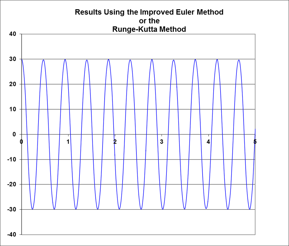
Here the oscillatory motion is clearly sinusoidal, as it should be. The results for this particular problem are almost identical whether you use the improved Euler method or the Runge-Kutta method. Since for this problem the results of both methods are virtually the same, you can save computational time and memory using the improved Euler method versus the Runge-Kutta method. This can be a significant advantage for real-time games. Remember the Runge-Kutta method requires four derivative computations per time step.
These methods aren’t the only ones at your disposal, but they are the most common. The Runge-Kutta method is particularly popular as a general-purpose numerical integration scheme. Other methods attempt to improve computational efficiency even further—that is, they are designed to minimize truncation error while still allowing you to take relatively large step sizes so as to reduce the number of steps you have to take in your integration. Still other methods are especially tailored for specific problem types. We cite some pretty good references for further reading on this subject in the Bibliography.
Summary
At this point you should be comfortable with the terms that appear in the equations of motion and be able to calculate terms like the sum of forces and moments, mass, and inertia. You should also have a solid understanding of basic numerical integration techniques. Implementing these techniques in code is really straightforward since they are composed of simple polynomial functions. The hard part is developing the derivative function for your problem. In the case of the equations of motion, the derivative function will include all your force and moment calculations for the particle or rigid body that you are modeling. You’ll see some more numerical integration code when you get to Chapter 8, Chapter 9, and Chapter 11.