
Chapter 2. Kinematics
In this chapter we’ll explain the fundamental aspects of the subject of kinematics. Specifically, we’ll explain the concepts of linear and angular displacement, velocity, and acceleration. We’ve prepared an example program for this chapter that shows you how to implement the kinematic equations for particle motion. After discussing particle motion, we go on to explain the specific aspects of rigid-body motion. This chapter, along with the next chapter on force, is prerequisite to understanding the subject of kinetics, which you’ll study in Chapter 4.
In the preface, we told you that kinematics is the study of the motion of bodies without regard to the forces acting on the body. Therefore, in kinematics, attention is focused on position, velocity, and acceleration of a body, how these properties are related, and how they change over time.
Here you’ll look at two types of bodies, particles and rigid bodies. A rigid body is a system of particles that remain at fixed distances from one another with no relative translation or rotation among them. In other words, a rigid body does not change its shape as it moves—or any changes in its shape are so small or unimportant that they can safely be neglected. When you are considering a rigid body, its dimensions and orientation are important, and you must account for both the body’s linear motion and its angular motion.
A particle, on the other hand, is a body that has mass but whose dimensions are negligible or unimportant in the problem being investigated. For example, when considering the path of a projectile or a rocket over a great distance, you can safely ignore the body’s dimensions when analyzing its trajectory. When you are considering a particle, its linear motion is important, but the angular motion of the particle itself is not. Think of it this way: when looking at a particle, you are zooming way out to view the big picture, so to speak, as opposed to zooming in as you do when looking at the rotation of rigid bodies.
Whether you are looking at problems involving particles or rigid bodies, there are some important kinematic properties common to both. These are, of course, the object’s position, velocity, and acceleration. The next section discusses these properties in detail.
Velocity and Acceleration
In general, velocity is a vector quantity that has magnitude and direction. The magnitude of velocity is speed. Speed is a familiar term—it’s how fast your speedometer says you’re going when driving your car down the highway. Formally, speed is the rate of travel, or the ratio of distance traveled to the time it took to travel that distance. In math terms, you can write:
| v = Δs/Δt |
where v is speed, the magnitude of velocity v, and Δs is distance traveled over the time interval Δt. Note that this relation reveals that the units for speed are composed of the basic dimension’s length divided by time, L/T. Some common units for speed are meters per second, m/s; feet per second, ft/sec; and miles per hour, mi/hr.
Here’s a simple example (illustrated in Figure 2-1): a car is driving down a straight road and passes marker one at time t1 and marker two at time t2, where t1 equals 0 seconds and t2 equals 1.136 seconds. The distance between these two markers, s, is 30 m. Calculate the speed of the car.
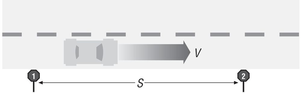
You are given that s equals 30 m; therefore, Δs equals 30 m and Δt equals t2 − t1 or 1.136 seconds. The speed of the car over this distance is:
| v = Δs/Δt = 30 m/1.136 sec = 26.4 m/sec |
which is approximately 60 mi/hr. This is a simple one-dimensional example, but it brings up an important point, which is that the speed just calculated is the average speed of the car over that distance. You don’t know anything at this point about the car’s acceleration, or whether or not it is traveling at a constant 60 mi/hr. It could very well be that the car was accelerating (or decelerating) over that 30 m distance.
To more precisely analyze the motion of the car in this example, you need to understand the concept of instantaneous velocity. Instantaneous velocity is the specific velocity at a given instant in time, not over a large time interval as in the car example. This means that you need to look at very small Δt’s. In math terms, you must consider the limit as Δt approaches 0—that is, as Δt gets infinitesimally small. This is written as follows:
| v = limΔt→0 (Δs/Δt) |
In differential terms, velocity is the derivative of displacement (change in position) with respect to time:
| v = ds/dt |
You can rearrange this relationship and integrate over the intervals from s1 to s2 and t1 to t2, as shown here:
| v dt = ds |
| ∫(s1 to s2) ds = ∫(t1 to t2) v dt |
| s2 – s1 = Δs = ∫(t1 to t2) v dt |
This relation shows that displacement is the integral of velocity over time. This gives you a way of working back and forth between displacement and velocity.
Kinematics makes an important distinction between displacement and distance traveled. In one dimension, displacement is the same as distance traveled; however, with vectors in space, displacement is actually the vector from the initial position to the final position without regard to the path traveled, while displacement is the difference between the starting position coordinates and the ending position coordinates. Thus, you need to be careful when calculating average velocity given displacement if the path from the starting position to the final position is not a straight line. When Δt is very small (as it approaches 0), displacement and distance traveled are the same.
Another important kinematic property is acceleration, which should also be familiar to you. Referring to your driving experience, you know that acceleration is the rate at which you can increase your speed. Your friend who boasts that his brand new XYZ 20II can go from 0 to 60 in 4.2 seconds is referring to acceleration. Specifically, he is referring to average acceleration.
Formally, average acceleration is the rate of change in velocity, or Δv over Δt:
| a = Δv/Δt |
Taking the limit as Δt goes to 0 gives the instantaneous acceleration:
| a = limΔt→0 Δv/Δt |
| a = dv/dt |
Thus, acceleration is the time rate of change in velocity, or, the derivative of velocity with respect to time.
Multiplying both sides by dt and integrating yields:
| dv = a dt |
| ∫(v1 to v2) dv = ∫(t1 to t2) a dt |
| v2 – v1 = Δv = ∫(t1 to t2) a dt |
This relationship provides a means to work back and forth between velocity and acceleration.
Thus, the relationships between displacement, velocity, and acceleration are:
| a = dv/dt = d2s/dt2 |
and:
| v dv = a ds |
This is the kinematic differential equation of motion (see the sidebar Second Derivatives for some helpful background). In the next few sections you’ll see some examples of the application of these equations for some common classes of problems in kinematics.
Constant Acceleration
One of the simplest classes of problems in kinematics involves constant acceleration. A good example of this sort of problem involves the acceleration due to gravity, g, on objects moving relatively near the earth’s surface, where the gravitational acceleration is a constant 9.81 m/s2. Having constant acceleration makes integration over time relatively easy since you can pull the acceleration constant out of the integrand, leaving just dt.
Integrating the relationship between velocity and acceleration described earlier when acceleration is constant yields the following equation for instantaneous velocity:
| ∫(v1 to v2) dv = ∫(t1 to t2) a dt |
| ∫(v1 to v2) dv = a ∫(t1 to t2) dt |
| v2 – v1 = a ∫(t1 to t2) dt |
| v2 – v1 = a (t2 − t1) |
| v2 = a t2 − a t1 + v1 |
When t1 equals 0, you can rewrite this equation in the following form:
| v2 = a t2 + v1 |
| v2 = v1 + a t2 |
This simple equation allows you to calculate the instantaneous velocity at any given time by knowing the elapsed time, the initial velocity, and the constant acceleration.
You can also derive an equation for velocity as a function of displacement instead of time by considering the kinematic differential equation of motion:
| v dv = a ds |
Integrating both sides of this equation yields the following alternative function for instantaneous velocity:
| ∫(v1 to v2) v dv = a ∫(s1 to s2) ds |
| (v22 − v12) / 2 = a (s2 − s1) |
| v22 = 2a (s2 − s1) + v12 |
You can derive a similar formula for displacement as a function of velocity, acceleration, and time by integrating the differential equation:
| v dt = ds |
with the formula derived earlier for instantaneous velocity:
| v2 = v1 + at |
substituted for v. Doing so yields the formula:
| s2 = s1 + v1 t + (a t2) / 2 |
In summary, the three preceding kinematic equations derived are:
| v2 = v1 + a t2 |
| v22 = 2a (s2 − s1) + v12 |
| s2 = s1 + v1 t + (a t2) / 2 |
Remember, these equations are valid only when acceleration is constant. Note that acceleration can be 0 or even negative in cases where the body is decelerating.
You can rearrange these equations by algebraically solving for different variables, and you can also derive other handy equations using the approach that we just demonstrated. For your convenience, we’ve provided some other useful kinematic equations for constant acceleration problems in Table 2-1.
To find: | Given these: | Use this: |
a | Δt, v1, v2 | a = (v2 – v1) / Δt |
a | Δt, v1, Δs | a = (2 Δs – 2 v1 Δt) / (Δt)2 |
a | v1, v2, Δs | a = (v22 – v12) / (2 Δs) |
Δs | a, v1, v2 | Δs = (v22 – v12) / (2a) |
Δs | Δt, v1, v2 | Δs = (Δt / 2) (v1 + v2) |
Δt | a, v1, v2 | Δt = (v2 – v1) / a |
Δt | a, v1, Δs | Δt = |
Δt | v1, v2, Δs | Δt =(2Δs) / (v1 + v2) |
v1 | Δt, a, v2 | v1 = v2 – aΔt |
v1 | Δt, a, Δs | v1 = Δs/Δt – (aΔt)/2 |
v1 | a, v2, Δs | v1 = |
In cases where acceleration is not constant, but is some function of time, velocity, or position, you can substitute the function for acceleration into the differential equations shown earlier to derive new equations for instantaneous velocity and displacement. The next section considers such a problem.
Nonconstant Acceleration
A common situation that arises in real-world problems is when drag forces act on a body in motion. Typically, drag forces are proportional to velocity squared. Recalling the equation of Newton’s second law of motion, F = ma, you can deduce that the acceleration induced by these drag forces is also proportional to velocity squared
Later we’ll show you some techniques to calculate this sort of drag force, but for now let the functional form of drag-induced acceleration be:
| a = –kv2 |
where k is a constant and the negative sign indicates that this acceleration acts in the direction opposing the body’s velocity. Now substituting this formula for acceleration into the previous equation and then rearranging yields:
| a = dv/dt |
| –kv2 = dv/dt |
| –k dt = dv/v2 |
If you integrate the right side of this equation from v1 to v2 and the left side from 0 to t, and then solve for v2, you’ll get this formula for the instantaneous velocity as a function of the initial velocity and time:
| –k ∫(0 to t) dt = ∫(v1 to v2) (1/v2) dv |
| –k t = 1/v1 – 1/v2 |
| v2 = v1 / (1 + v1k t) |
If you substitute this equation for v in the relation v = ds/dt and integrate again, you’ll end up with a new equation for displacement as a function of initial velocity and time; see the following procedure:
| v dt = ds; where v = v1 / (1 + v1k t) |
| ∫(0 to t) v dt = ∫(s1 to s2) ds |
| ∫(0 to t) [v1 / (1 + v1k t)] dt = ∫(s1 to s2) ds |
| ln(1 + v1 k t) / k = s2 – s1 |
If s1 equals 0, then:
| s = ln(1 + v1 k t) / k |
Note that in this equation, ln is the natural logarithm operator.
This example demonstrates the relative complexity of nonconstant acceleration problems versus constant acceleration problems. It’s a fairly simple example where you are able to derive closed-form equations for velocity and displacement. In practice, however, there may be several different types of forces acting on a given body in motion, which could make the expression for induced acceleration quite complicated. This complexity would render a closed-form solution like the preceding one impossible to obtain unless you impose some simplifying restrictions on the problem, forcing you to rely on other solution techniques like numerical integration. We’ll talk about this sort of problem in greater depth in Chapter 11.
2D Particle Kinematics
When we are considering motion in one dimension—that is, when the motion is restricted to a straight line—it is easy enough to directly apply the formulas derived earlier to determine instantaneous velocity, acceleration, and displacement. However, in two dimensions, with motion possible in any direction on a given plane, you must consider the kinematic properties of velocity, acceleration, and displacement as vectors.
Using rectangular coordinates in the standard Cartesian coordinate system, you must account for the x and y components of displacement, velocity, and acceleration. Essentially, you can treat the x and y components separately and then superimpose these components to define the corresponding vector quantities.
To help keep track of these x and y components, let i and j be unit vectors in the x- and y-directions, respectively. Now you can write the kinematic property vectors in terms of their components as follows:
| v = vx i + vy j |
| a = ax i + ay j |
If x is the displacement in the x-direction and y is the displacement in the y-direction, then the displacement vector is:
| s = x i + y j |
It follows that:
| v = ds/dt = dx/dt i + dy/dt j |
| a = dv/dt = d2s/dt2 = d2x/dt2 i + d2y/dt2 j |
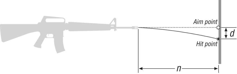
Consider a simple example where you’re writing a shooting game and you need to figure out the vertical drop in a fired bullet from its aim point to the point at which it actually hits the target. In this example, assume that there is no wind and no drag on the bullet as it flies through the air (we’ll deal with wind and drag on projectiles in Chapter 6). These assumptions reduce the problem to one of constant acceleration, which in this case is that due to gravity. It is this gravitational acceleration that is responsible for the drop in the bullet as it travels from the rifle to the target. Figure 2-2 illustrates the problem.
Note
While we’re talking about guns and shooting here, we should point out that these techniques can be applied just as easily to simulating the flight of angry birds in Angry Birds being shot from oversized slingshots, as in the very popular iPhone app. Heck, you can use these techniques to simulate flying monkeys, ballistic shoes, or coconuts being hurled at Navy combatants! This particle kinematic stuff is perfect for diversionary smartphone apps.
Let the origin of the 2D coordinate system be at the end of the rifle with the x-axis pointing toward the target and the y-axis pointing up. Positive displacements along the x-axis are toward the target, and positive displacements along the y-axis are upward. This implies that the gravitational acceleration will act in the negative y-direction.
Treating the x and y components separately allows you to break up the problem into small, easy-to-manage pieces. Looking at the x component first, you know that the bullet will leave the rifle with an initial muzzle velocity vm in the x-direction, and since we are neglecting drag, this speed will be constant. Thus:
| ax = 0 |
| vx = vm |
| x = vx t = vm t |
Now looking at the y component, you know that the initial speed in the y-direction, as the bullet leaves the rifle, is 0, but the y-acceleration is –g (due to gravity). Thus:
| ay = –g = dvy/dt |
| vy = ay t = –g t |
| y = (1/2) ay t2 = –(1/2) g t2 |
The displacement, velocity, and acceleration vectors can now be written as:
| s = (vm t) i – (1/2 g t2) j |
| v = (vm) i – (g t) j |
| a = – (g) j |
These equations give the instantaneous displacement, velocity, and acceleration for any given instant between the time the bullet leaves the rifle and the time it hits the target. The magnitudes of these vectors give the total displacement, velocity, and acceleration at a given time. For example:
To calculate the bullet’s vertical drop at the instant the bullet hits the target, you must first calculate the time required to reach the target; then, you can use that time to calculate the y component of displacement, which is the vertical drop. Here are the formulas to use:
| thit = xhit/vm = n/vm |
| d = yhit = –(1/2) g (thit)2 |
where n is the distance from the rifle to the target and d is the vertical drop of the bullet at the target.
If the distance to the target, n, equals 500 m and the muzzle velocity, vm, equals 800 m/sec, then the equations for thit and d give:
| thit = 0.625 sec |
| d = 1.9 m |
These results tell you that in order to hit the intended target at that range, you’ll need to aim for a point about 2 m above it.
3D Particle Kinematics
Extending the kinematic property vectors to three dimensions is not very difficult. It simply involves the addition of one more component to the vector representations shown in the previous section on 2D kinematics. Introducing k as the unit vector in the z-direction, you can now write:
| s = x i + y j + z k |
| v = ds/dt = dx/dt i + dy/dt j + dz/dt k |
| a = d2s/dt2 = d2x/dt2 i + d2y/dt2 j + d2z/dt2 k |
Instead of treating two components separately and then superimposing them, you now treat three components separately and superimpose these. This is best illustrated by an example.
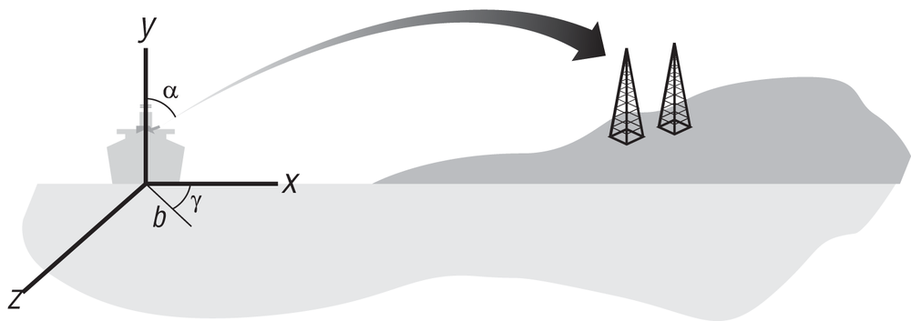
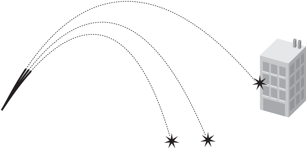
Suppose that instead of a hunting game, you’re now writing a game that involves the firing of a cannon from, say, a battleship to a target some distance away—for example, another ship or an inland target like a building. To add complexity to this activity for your user, you’ll want to give her control of several factors that affect the shell’s trajectory—namely, the firing angle of the cannon, both horizontal and vertical angles, and the muzzle velocity of the shell, which is controlled by the amount of powder packed behind the shell when it’s loaded into the cannon. The situation is set up in Figure 2-3.
We’ll show you how to set up the kinematic equations for this problem by treating each vector component separately at first and then combining these components.
X Components
The x components here are similar to those in the previous section’s rifle example in that there is no drag force acting on the shell; thus, the x component of acceleration is 0, which means that the x component of velocity is constant and equal to the x component of the muzzle velocity as the shell leaves the cannon. Note that since the cannon barrel may not be horizontal, you’ll have to compute the x component of the muzzle velocity, which is a function of the direction in which the cannon is aimed.
The muzzle velocity vector is:
| vm = vmx i + vmy j + vmz k |
and you are given only the direction of vm as determined by the direction in which the user points the cannon, and its magnitude as determined by the amount of powder the user packs into the cannon. To calculate the components of the muzzle velocity, you need to develop some equations for these components in terms of the direction angles of the cannon and the magnitude of the muzzle velocity.
You can use the direction cosines of a vector to determine the velocity components as follows:
| cos θx = vmx/vm |
| cos θy = vmy/vm |
| cox θz = vmz/vm |
Refer to Appendix A for a description and illustration of vector direction cosines.
Since the initial muzzle velocity vector direction is the same as the direction in which the cannon is aimed, you can treat the cannon as a vector with a magnitude of L, its length, and pointing in a direction defined by the angles given in this problem. Using the cannon length, L, and its components instead of muzzle velocity in the equations for direction cosines gives:
| cos θx = Lx/L |
| cos θy = Ly/L |
| cos θz = Lz/L |
In this example, you are given the angles α and γ (see Figure 2-4) that define the cannon orientation.
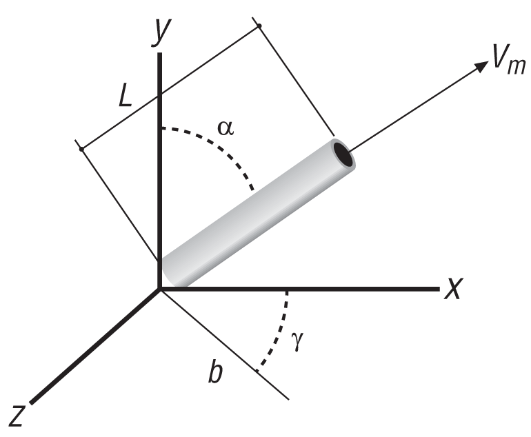
Using these angles, it follows that the projection, b, of the cannon length, L, onto the x-z plane is:
| b = L cos(90° – α) |
and the components of the cannon length, L, on each coordinate axis are:
| Lx = b cos γ |
| Ly = L cos α |
| Lz = b sin γ |
Now that you have the information required to compute direction cosines, you can write equations for the initial muzzle velocity components as follows:
| vmx = vm cos θx |
| vmy = vm cos θy |
| vmz = vm cos θz |
Finally, you can write the x components of displacement, velocity, and acceleration as follows:
| ax = 0 |
| vx = vmx = vm cos θx |
| x = vx t = (vm cos θx) t |
Y Components
The y components are just like the previous rifle example, again with the exception here of the initial velocity in the y-direction:
| vmy = vm cos θy |
Thus:
| ay = –g |
| vy = vmy + a t = (vm cos θy) – g t |
Before writing the equation for the y component of displacement, you need to consider the elevation of the base of the cannon, plus the height of the end of the cannon barrel, in order to calculate the initial y component of displacement when the shell leaves the cannon. Let yb be the elevation of the base of the cannon, and let L be the length of the cannon barrel; then the initial y component of displacement, yo, is:
| yo = yb + L cos α |
Now you can write the equation for y as:
| y = yo + vmy t + (1/2) a t2 |
| y = (yb + L cos α) + (vm cos θy) t – (1/2) g t2 |
Z Components
The z components are largely analogous to the x components and can be written as follows:
| az = 0 |
| vz = vmz = vm cos θz |
| z = vz t = (vm cos θz) t |
The Vectors
With the components all worked out, you can now combine them to form the vector for each kinematic property. Doing so for this example gives the displacement, velocity, and acceleration vectors shown here:
| s = [(vm cos θx) t] i + [(yb + L cos α) + (vm cos θy) t – (1/2) g t2] j + [(vm cos θz) t ] k |
| v = [vm cos θx ] i + [(vm cos θy) – g t ] j + [vm cos θz ] k |
| a = –g j |
Observe here that the displacement vector essentially gives the position of the shell’s center of mass at any given instant in time; thus, you can use this vector to plot the shell’s trajectory from the cannon to the target.
Hitting the Target
Now that you have the equations fully describing the shell’s trajectory, you need to consider the location of the target in order to determine when a direct hit occurs. To show you how to do this, we’ve prepared a sample program that implements these kinematic equations along with a simple bounding box collision detection method for checking whether or not the shell has struck the target. Basically, at each time step where we calculate the position of the shell after it has left the cannon, we check to see if this position falls within the bounding dimensions of the target object represented by a cube.
The sample program is set up such that you can change all of the variables in the simulation and view the effects of your changes. Figure 2-5 shows the main screen for the cannon example program, with the governing variables shown on the left. The upper illustration is a bird’s-eye view looking down on the cannon and the target, while the lower illustration is a profile (side) view.
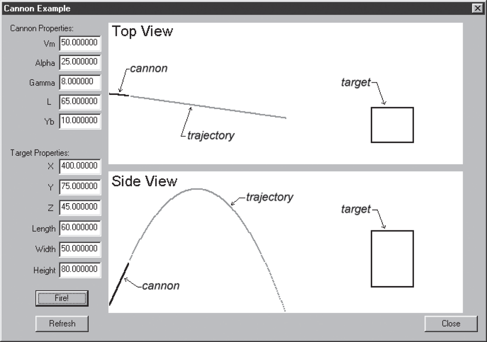
You can change any of the variables shown on the main window and press the Fire button to see the resulting flight path of the shell. A message box will appear when you hit the target or when the shell hits the ground. The program is set up so you can repeatedly change the variables and press Fire to see the result without erasing the previous trial. This allows you to gauge how much you need to adjust each variable in order to hit the target. Press the Refresh button to redraw the views when they get too cluttered.
Figure 2-6 shows a few trial shots that we made before finally hitting the target.
The code for this example is really quite simple. Aside from the overhead of the window, controls, and illustrations setup, all of the action takes place when the Fire button is pressed. In pseudocode, the Fire button’s pressed event handler looks something like this:
    FIRE BUTTON PRESSED EVENT:

        Fetch and store user input values for global variables,
        Vm, Alpha, Gamma, L, Yb, X, Y, Z, Length, Width, Height...

        Initialize the time and status variables...
        status = 0;
        time = 0;

        Start stepping through time for the simulation
        until the target is hit, the shell hits
        the ground, or the simulation times out...

        while(status == 0)
        {
            // do the next time step
            status = DoSimulation();

            Update the display...

        }

        // Report results
        if (status == 1)
            Display DIRECT HIT message to the user...

        if (status == 2)
            Display MISSED TARGET message to the user...

        if (status == 3)
            Display SIMULATION TIMED OUT message to the user...
The first task is to simply get the new values for the variables
shown on the main window. After that, the program enters a while loop, stepping through increments of
time and recalculating the position of the shell projectile using the
formula for the displacement vector, s, shown earlier. The shell position at the
current time is calculated in the function DoSimulation. Immediately after calling
DoSimulation, the program updates the
illustrations on the main window, showing the shell’s trajectory.
DoSimulation returns 0, keeping the while loop going, if there has not yet been a
collision or if the time has not yet reached the preset time-out
value.
Once the while loop terminates
by DoSimulation returning nonzero,
the program checks the return value from this function call to see if a
hit has occurred between the shell and the ground or the shell and the
target. Just so the program does not get stuck in this while loop, DoSimulation will return a value of 3, indicating that it is taking too
long.
Now let’s look at what’s happing in the function DoSimulation (we’ve also included here the
global variables that are used in DoSimulation).
//---------------------------------------------------------------------------//
// Define a custom type to represent
// the three components of a 3D vector, where
// i represents the x component, j represents
// the y component, and k represents the z
// component
//---------------------------------------------------------------------------//
typedef struct TVectorTag
{
     double i;
     double j;
     double k;
} TVector;

//---------------------------------------------------------------------------//
// Now define the variables required for this simulation
//---------------------------------------------------------------------------//
double          Vm;    // Magnitude of muzzle velocity, m/s
double          Alpha; // Angle from y-axis (upward) to the cannon.
                       // When this angle is 0, the cannon is pointing
                       // straight up, when it is 90 degrees, the cannon
                       // is horizontal
double          Gamma; // Angle from x-axis, in the x-z plane to the cannon.
                       // When this angle is 0, the cannon is pointing in
                       // the positive x-direction, positive values of this angle
                       // are toward the positive z-axis
double          L;     // This is the length of the cannon, m
double          Yb;    // This is the base elevation of the cannon, m

double          X;     // The x-position of the center of the target, m
double          Y;     // The y-position of the center of the target, m
double          Z;     // The z-position of the center of the target, m
double          Length; // The length of the target measured along the x-axis, m
double          Width;  // The width of the target measured along the z-axis, m
double          Height; // The height of the target measure along the y-axis, m

TVector          s;     // The shell position (displacement) vector

double          time;   // The time from the instant the shell leaves
                        // the cannon, seconds
double          tInc;   // The time increment to use when stepping through
                        // the simulation, seconds

double          g;      // acceleration due to gravity, m/s^2

//-----------------------------------------------------------------------------//
// This function steps the simulation ahead in time. This is where the kinematic
// properties are calculated. The function will return 1 when the target is hit,
// and 2 when the shell hits the ground (x-z plane) before hitting the target;
// otherwise, the function returns 0.
//-----------------------------------------------------------------------------//
int    DoSimulation(void)
//-----------------------------------------------------------------------------//
{
    double    cosX;
    double    cosY;
    double    cosZ;
    double    xe, ze;
    double    b, Lx, Ly, Lz;
    double    tx1, tx2, ty1, ty2, tz1, tz2;

    // step to the next time in the simulation
    time+=tInc;

    // First calculate the direction cosines for the cannon orientation.
    // In a real game, you would not want to put this calculation in this
    // function since it is a waste of CPU time to calculate these values
    // at each time step as they never change during the sim. We only put them
     // here in this case so you can see all the calculation steps in a single
    // function.
    b = L * cos((90-Alpha) *3.14/180);  // projection of barrel onto x-z plane
    Lx = b * cos(Gamma * 3.14/180);    // x-component of barrel length
    Ly = L * cos(Alpha * 3.14/180);    // y-component of barrel length
    Lz = b  * sin(Gamma * 3.14/180);    // z-component of barrel length

    cosX = Lx/L;
    cosY = Ly/L;
    cosZ = Lz/L;

    // These are the x and z coordinates of the very end of the cannon barrel
    // we'll use these as the initial x and z displacements
    xe = L * cos((90-Alpha) *3.14/180) * cos(Gamma * 3.14/180);
    ze = L * cos((90-Alpha) *3.14/180) * sin(Gamma * 3.14/180);

    // Now we can calculate the position vector at this time
    s.i =     Vm * cosX * time + xe;
    s.j =     (Yb + L * cos(Alpha*3.14/180)) + (Vm * cosY * time) −
        (0.5 * g * time * time);
    s.k =     Vm * cosZ * time + ze;

    // Check for collision with target
    // Get extents (bounding coordinates) of the target
    tx1 = X - Length/2;
    tx2 = X + Length/2;
    ty1 = Y - Height/2;
    ty2 = Y + Height/2;
    tz1 = Z - Width/2;
    tz2 = Z + Width/2;

    // Now check to see if the shell has passed through the target
    // We're using a rudimentary collision detection scheme here where
    // we simply check to see if the shell's coordinates are within the
    // bounding box of the target. This works for demo purposes, but
    // a practical problem is that you may miss a collision if for a given
    // time step the shell's change in position is large enough to allow
    // it to "skip" over the target.
    // A better approach is to look at the previous time step's position data
    // and to check the line from the previous position to the current position
    // to see if that line intersects the target bounding box.
    if( (s.i >= tx1 && s.i <= tx2) &&
        (s.j >= ty1 && s.j <= ty2) &&
        (s.k >= tz1 && s.k <= tz2) )
        return 1;

    // Check for collision with ground (x-z plane)
    if(s.j <= 0)
        return 2;

    // Cut off the simulation if it's taking too long
    // This is so the program does not get stuck in the while loop
    if(time>3600)
        return 3;

    return 0;
}
We’ve commented the code so that you can readily see what’s going on. This function essentially does four things: 1) increments the time variable by the specified time increment, 2) calculates the initial muzzle velocity components in the x-, y-, and z-directions, 3) calculates the shell’s new position, and 4) checks for a collision with the target using a bounding box scheme or the ground.
Here’s the code that computes the shell’s position:
    // Now we can calculate the position vector at this time
    s.i =     Vm * cosX * time + xe;
    s.j =     (Yb + L * cos(Alpha*3.14/180)) + (Vm * cosY * time) −
        (0.5 * g * time * time);
    s.k =     Vm * cosZ * time + ze;
This code calculates the three components of the displacement vector, s, using the formulas that we gave you earlier. If you wanted to compute the velocity and acceleration vectors as well, just to see their values, you should do so in this section of the program. You can set up a couple of new global variables to represent the velocity and acceleration vectors, just as we did with the displacement vector, and apply the velocity and acceleration formulas that we gave you.
That’s all there is to it. It’s obvious by playing with this sample program that the shell’s trajectory is parabolic in shape, which is typical projectile motion. We’ll take a more detailed look at this sort of motion in Chapter 6.
Even though we put a comment in the source code, we must reiterate a warning here regarding the collision detection scheme that we used in this example. Because we’re checking only the current position coordinate to see if it falls within the bounding dimensions of the target cube, we run the risk of skipping over the target if the change in position is too large for a given time step. A better approach would be to keep track of the shell’s previous position and check to see if the line connecting the previous position to the new one intersects the target cube.
Kinematic Particle Explosion
At this point you might be wondering how particle kinematics can help you create realistic game content unless you’re writing a game that involves shooting a gun or a cannon. If so, let us offer you a few ideas and then show you an example. Say you’re writing a football simulation game. You can use particle kinematics to model the trajectory of the football after it’s thrown or kicked. You can also treat the wide receivers as particles when calculating whether or not they’ll be able to catch the thrown ball. In this scenario you’ll have two particles—the receiver and the ball—traveling independently, and you’ll have to calculate when a collision occurs between these two particles, indicating a catch (unless, of course, your player is all thumbs and fumbles the ball after it hits his hands). You can find similar applications for other sports-based games as well.
What about a 3D “shoot ’em up” game? How could you use particle kinematics in this genre aside from bullets, cannons, grenades, and the like? Well, you could use particle kinematics to model your player when she jumps into the air, either from a run or from a standing position. For example, your player reaches the middle of a catwalk only to find a section missing, so you immediately back up a few paces to get a running head start before leaping into the air, hoping to clear the gap. This long-jump scenario is perfect for using particle kinematics. All you really need to do is define your player’s initial velocity, both speed and take-off angle, and then apply the vector formula for displacement to calculate whether or not the player makes the jump. You can also use the displacement formula to calculate the player’s trajectory so that you can move the player’s viewpoint accordingly, giving the illusion of leaping into the air. You may in fact already be using these principles to model this action in your games, or at least you’ve seen it done if you play games of this genre. If your player happens to fall short on the jump, you can use the formulas for velocity to calculate the player’s impact velocity when she hits the ground below. Based on this impact velocity, you can determine an appropriate amount of damage to deduct from the player’s health score, or if the velocity is over a certain threshold, you can say goodbye to your would-be adventurer!
Another use for simple particle kinematics is for certain special effects like particle explosions. This sort of effect is quite simple to implement and really adds a sense of realism to explosion effects. The particles don’t just fly off in random, straight-line trajectories. Instead, they rise and fall under the influence of their initial velocity, angle, and the acceleration due to gravity, which gives the impression that the particles have mass.
So, let’s explore an example of a kinematic particle explosion. The code for this example is taken from the cannon example discussed previously, so a lot of it should look familiar to you. Figure 2-7 shows this example program’s main window.
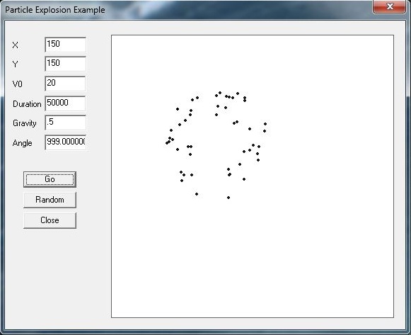
The explosion effect takes place in the large rectangular area on the right. While the black dots representing exploding particles are certainly static in the figure, we assure you they move in the most spectacular way during the simulation.
In the edit controls on the left, you specify an x- and y-position for the effect, along with the initial velocity of the particles (which is a measure of the explosion’s strength), a duration in milliseconds, a gravity factor, and finally an angle. The angle parameter can be any number between 0 and 360 degrees or 999. When you specify an angle in the range of 0 to 360 degrees, all the particles in the explosion will be launched generally in that direction. If you specify a value of 999, then all the particles will shoot off in random directions. The duration parameter is essentially the life of the effect. The particles will fade out as they approach that life.
The first thing you need to do for this example is set up some structures and global variables to represent the particle effect and the individual particles making up the effect along with the initial parameters describing the behavior of the effect as discussed in the previous paragraph. Here’s the code:
//---------------------------------------------------------------------------//
// Define a custom type to represent each particle in the effect.
//---------------------------------------------------------------------------//
typedef     struct _TParticle
{
     float          x;           // x coordinate of the particle
     float          y;           // y coordinate of the particle
     float          vi;          // initial velocity
     float          angle;       // initial trajectory (direction)
     int            life;        // duration in milliseconds
     int            r;           // red component of particle's color
     int            g;           // green component of particle's color
     int            b;           // blue component of particle's color
     int            time;        // keeps track of the effect's time
     float          gravity;     // gravity factor
     BOOL           Active;      // indicates whether this particle
                                 // is active or dead
} TParticle;

#define     _MAXPARTICLES 50

typedef struct _TParticleExplosion
{
     TParticle     p[_MAXPARTICLES];  // list of particles
                                      // making up this effect
     int           V0; // initial velocity, or strength, of the effect
     int           x;  // initial x location
     int           y;  // initial y location
     BOOL          Active;      // indicates whether this effect is
                                //active or dead
} TParticleExplosion;

//---------------------------------------------------------------------------//
// Now define the variables required for this simulation
//---------------------------------------------------------------------------//
TParticleExplosion     Explosion;

int                      xc;         // x coordinate of the effect
int                      yc;         // y coordinate of the effect
int                      V0;         // initial velocity
int                      Duration;   // life in milliseconds
float                    Gravity;    // gravity factor (acceleration)
float                    Angle;      // indicates particles' direction
You can see from this code that the particle explosion effect is made up of a collection of particles. The behavior of each particle is determined by kinematics and the initial parameters set for each particle.
Whenever you press the Go button, the initial parameters that you
specified are used to initialize the particle explosion (if you press the
Random button, the program randomly selects these initial values for you).
This takes place in the function called CreateParticleExplosion:
/////////////////////////////////////////////////////////////////////
/*     This function creates a new particle explosion effect.

     x,y:      starting point of the effect
     Vinit:    a measure of how fast the particles will be sent flying
               (it's actually the initial velocity of the particles)
     life:     life of the particles in milliseconds; particles will
               fade and die out as they approach
               their specified life
     gravity:  the acceleration due to gravity, which controls the
               rate at which particles will fall
               as they fly
     angle:    initial trajectory angle of the particles,
               specify 999 to create a particle explosion
               that emits particles in all directions; otherwise,
               0 right, 90 up, 180 left, etc...
*/
void CreateParticleExplosion(int x, int y, int Vinit, int life,
                             float gravity, float angle)
{
     int   i;
     int   m;
     float f;

     Explosion.Active = TRUE;
     Explosion.x = x;
     Explosion.y = y;
     Explosion.V0 = Vinit;

     for(i=0; i<_MAXPARTICLES; i++)
     {
          Explosion.p[i].x = 0;
          Explosion.p[i].y = 0;
          Explosion.p[i].vi = tb_Rnd(Vinit/2, Vinit);

          if(angle < 999)
          {
               if(tb_Rnd(0,1) == 0)
                    m = −1;
               else
                    m = 1;
               Explosion.p[i].angle = -angle + m * tb_Rnd(0,10);
          } else
               Explosion.p[i].angle = tb_Rnd(0,360);

          f = (float) tb_Rnd(80, 100) / 100.0f;
          Explosion.p[i].life = tb_Round(life * f);
          Explosion.p[i].r = 255;//tb_Rnd(225, 255);
          Explosion.p[i].g = 255;//tb_Rnd(85, 115);
          Explosion.p[i].b = 255;//tb_Rnd(15, 45);
          Explosion.p[i].time = 0;
          Explosion.p[i].Active = TRUE;
          Explosion.p[i].gravity = gravity;
     }

}
Here you can see that all the particles are set to start off in the
same position, as specified by the x and
y coordinates that you provide; however, you’ll
notice that the initial velocity of each particle is actually randomly
selected from a range of Vinit/2 to
Vinit. We do this to give the particle
behavior some variety. We do the same thing for the life parameter of each
particle so they don’t all fade out and die at the exact same time.
After the particle explosion is created, the program enters a loop
to propagate and draw the effect. The loop is a while loop, as shown here in pseudocode:
while(status)
{
    Clear the off screen buffer...

    status = DrawParticleExplosion( );

    Copy the off screen buffer to the screen...
}
The while loop continues as long
as status remains true, which indicates that the particle effect
is still alive. After all the particles in the effect reach their set
life, then the effect is dead and status will be set to false. All the calculations for the particle
behavior actually take place in the function called DrawParticleExplosion; the rest of the code in
this while loop is for clearing the
off-screen buffer and then copying it to the main window.
DrawParticleExplosion updates the
state of each particle in the effect by calling another function, UpdateParticleState, and then draws the effect
to the off-screen buffer passed in as a parameter. Here’s what these two
functions look like:
//---------------------------------------------------------------------------//
// Draws the particle system and updates the state of each particle.
// Returns false when all of the particles have died out.
//---------------------------------------------------------------------------//

BOOL     DrawParticleExplosion(void)
{
     int      i;
     BOOL     finished = TRUE;
     float    r;

     if(Explosion.Active)
       for(i=0; i<_MAXPARTICLES; i++)
       {
          if(Explosion.p[i].Active)
          {
               finished = FALSE;

               // Calculate a color scale factor to fade the particle's color
               // as its life expires
               r = ((float)(Explosion.p[i].life-
                     Explosion.p[i].time)/(float)(Explosion.p[i].life));

               ...
               Draw the particle as a small circle...
               ...

               Explosion.p[i].Active = UpdateParticleState(&(Explosion.p[i]),
                                                           10);
          }
       }

     if(finished)
          Explosion.Active = FALSE;

     return !finished;
}

//---------------------------------------------------------------------------//
/*  This is generic function to update the state of a given particle.
     p:         pointer to a particle structure
     dtime:     time increment in milliseconds to
                advance the state of the particle

     If the total elapsed time for this particle has exceeded the particle's
     set life, then this function returns FALSE, indicating that the particle
     should expire.
*/
BOOL     UpdateParticleState(TParticle* p, int dtime)
{
     BOOL retval;
     float     t;

     p->time+=dtime;
     t = (float)p->time/1000.0f;
     p->x = p->vi * cos(p->angle*PI/180.0f) * t;
     p->y = p->vi * sin(p->angle*PI/180.0f) * t + (p->gravity*t*t)/2.0f;

     if (p->time >= p->life)
          retval = FALSE;
     else
          retval = TRUE;

     return retval;
}
UpdateParticleState uses the
kinematic formulas that we’ve already shown you to update the particle’s
position as a function of its initial velocity, time, and the acceleration
due to gravity. After UpdateParticleState is called, DrawParticleExplosion scales down each
particle’s color, fading it to black, based on the life of each particle
and elapsed time. The fade effect is simply to show the particles dying slowly
over time instead of disappearing from the screen. The effect resembles
the behavior of fireworks as they explode in the night sky.
Rigid-Body Kinematics
The formulas for displacement, velocity, and acceleration discussed in the previous sections apply equally well for rigid bodies as they do for particles. The difference is that with rigid bodies, the point on the rigid body that you track, in terms of linear motion, is the body’s center of mass (gravity).
When a rigid body translates with no rotation, all of the particles making up the rigid body move on parallel paths since the body does not change its shape. Further, when a rigid body does rotate, it generally rotates about axes that pass through its center of mass, unless the body is hinged at some other point about which it’s forced to rotate. These facts make the center of mass a convenient point to use to track its linear motion. This is good news for you since you can use all of the material you learned on particle kinematics here in your study of rigid-body kinematics.
The procedure for dealing with rigid bodies involves two distinct aspects: 1) tracking the translation of the body’s center of mass, and 2) tracking the body’s rotation. The first aspect is old hat by now—just treat the body as a particle. The second aspect, however, requires you to consider a few more concepts—namely, local coordinates, angular displacement, angular velocity, and angular acceleration.
For most of the remainder of this chapter, we’ll discuss plane kinematics of rigid bodies. Plane motion simply means that the body’s motion is restricted to a flat plane in space where the only axis of rotation about which the body can rotate is perpendicular to the plane. Plane motion is essentially two-dimensional. This allows us to focus on the new kinematic concepts of angular displacement, velocity, and acceleration without getting lost in the math required to describe arbitrary rotation in three dimensions.
You might be surprised by how many problems lend themselves to plane kinematic solutions. For example, in some popular 3D “shoot ’em up” games, your character is able to push objects, such as boxes and barrels, around on the floor. While the game world here is three dimensions, these particular objects may be restricted to sliding on the floor—a plane—and thus can be treated like a 2D problem. Even if the player pushes on these objects at some angle instead of straight on, you’ll be able to simulate the sliding and rotation of these objects using 2D kinematics (and kinetics) techniques.
Local Coordinate Axes
Earlier, we defined the Cartesian coordinate system to use for your fixed global reference, or world coordinates. This world coordinate system is all that’s required when treating particles; however, for rigid bodies you’ll also use a set of local coordinates fixed to the body. Specifically, this local coordinate system will be fixed at the body’s center-of-mass location. You’ll use this coordinate system to track the orientation of the body as it rotates.
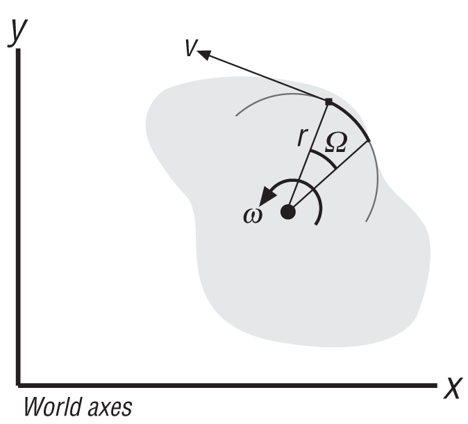
For plane motion, we require only one scalar quantity to describe the body’s orientation. This is illustrated in Figure 2-8.
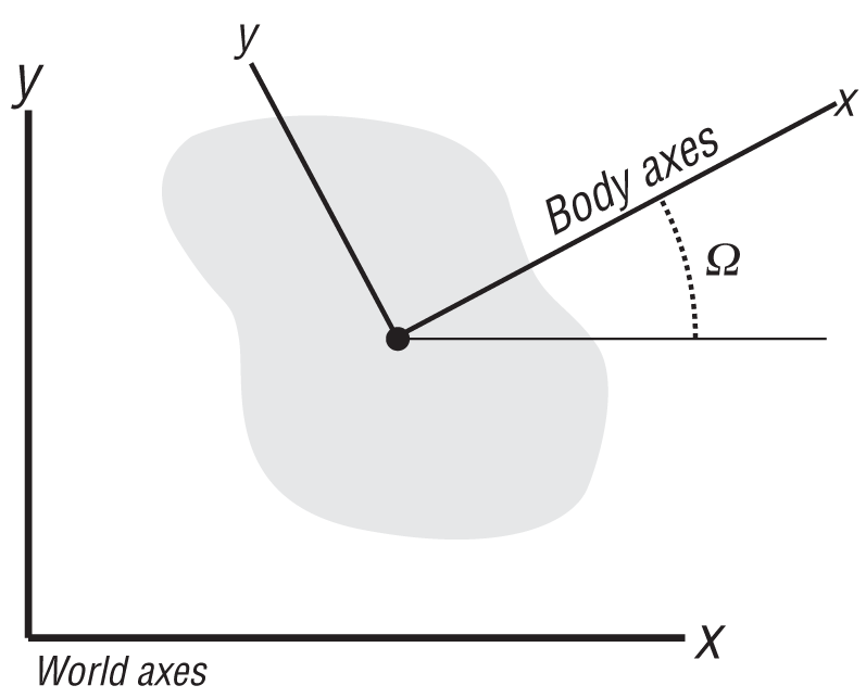
Here the orientation, Ω, is defined as the angular difference between the two sets of coordinate axes: the fixed world axes and the local body axes. This is the so-called Euler angle. In general 3D motion there is a total of three Euler angles, which are usually called yaw, pitch, and roll in aerodynamic and hydrodynamic jargon. While these angular representations are easy to visualize in terms of their physical meaning, they aren’t so nice from a numerical point of view, so you’ll have to look for alternative representations when writing your 3D real-time simulator. These issues are addressed in Chapter 9.
Angular Velocity and Acceleration
In two-dimensional plane motion, as the body rotates, Ω will change, and the rate at which it changes is the angular velocity, ω. Likewise, the rate at which ω changes is the angular acceleration, α. These angular properties are analogous to the linear properties of displacement, velocity, and acceleration. The units for angular displacement, velocity, and acceleration are radians (rad), radians per sec (rad/s), and radians per second-squared (rad/s2), respectively.
Mathematically, you can write these relations between angular displacement, angular velocity, and angular acceleration as:
| ω = dΩ/dt |
| α = dω/dt = d2Ω/dt2 |
| ω = ∫ α dt |
| Ω = ∫ ω dt |
| ω dω = α dΩ |
In fact, you can substitute the angular properties Ω, ω, and α for the linear properties s, v, and a in the equations derived earlier for particle kinematics to obtain similar kinematic equations for rotation. For constant angular acceleration, you’ll end up with the following equations:
| ω2 = ω1 + α t |
| ω22 = ω12 + 2 α (Ω2 − Ω1) |
| Ω2 = Ω1 + ω1t + (1/2) α t2 |
When a rigid body rotates about a given axis, every point on the rigid body sweeps out a circular path around the axis of rotation. You can think of the body’s rotation as causing additional linear motion of each particle making up the body—that is, this linear motion is in addition to the linear motion of the body’s center of mass. To get the total linear motion of any particle or point on the rigid body, you must be able to relate the angular motion of the body to the linear motion of the particle or point as it sweeps its circular path about the axis of rotation.
Before we show you how to do this, we’ll explain why you would even want to perform such a calculation. Basically, in dynamics, knowing that two objects have collided is not always enough, and you’ll often want to know how hard, so to speak, these two objects have collided. When you’re dealing with interacting rigid bodies that may at some point make contact with one another or with other fixed objects, you need to determine not only the location of the points of contact, but also the relative velocity or acceleration between the contact points. This information will allow you to calculate the interaction forces between the colliding bodies.
The arc length of the path swept by a particle on the rigid body is a function of the distance from the axis of rotation to the particle and the angular displacement, Ω. We’ll use c to denote arc length and r to denote the distance from the axis of rotation to the particle, as shown in Figure 2-9.
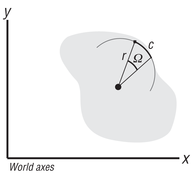
The formula relating arc length to angular displacement is:
| c = r Ω |
where Ω must be in radians, not degrees. If you differentiate this formula with respect to time:
| dc/dt = r dΩ/dt |
you get an equation relating the linear velocity of the particle as it moves along its circular path to the angular velocity of the rigid body. This equation is written as follows:
| v = r ω |
This velocity as a vector is tangent to the circular path swept by the particle. Imagine this particle as a ball at the end of a rod where the other end of the rod is fixed to a rotating axis. If the ball is released from the end of the rod as it rotates, the ball will fly off in a direction tangent to the circular path it was taking when attached to the rod. This is in the same direction as the tangential linear velocity given by the preceding equation. Figure 2-10 illustrates the tangential velocity.
Differentiating the equation, v = r ω:
| dv/dt = r dω/dt |
yields this formula for the tangential linear acceleration as a function of angular acceleration:
| at = r α |
Note that there is another component of acceleration for the particle that results from the rotation of the rigid body. This component—the centripetal acceleration—is normal, or perpendicular, to the circular path of the particle and is always directed toward the axis of rotation. Remember that velocity is a vector and since acceleration is the rate of change in the velocity vector, there are two ways that acceleration can be produced. One way is by a change in the magnitude of the velocity vector—that is, a change in speed—and the other way is a change in the direction of the velocity vector. The change in speed gives rise to the tangential acceleration component, while the direction change gives rise to the centripetal acceleration component. The resultant acceleration vector is the vector sum of the tangential and centripetal accelerations (see Figure 2-11). Centripetal acceleration is what you feel when you take your car around a tight curve even though your speed is constant.

The formula for the magnitude of centripetal acceleration, an, is:
| an = v2/r |
where v is the tangential velocity. Substituting the equation for tangential velocity into this equation for centripetal acceleration gives the following alternative form:
| an = r ω2 |
In two dimensions you can easily get away with using these scalar equations; however, in three dimensions you’ll have to use the vector forms of these equations. Angular velocity as a vector is parallel with the axis of rotation. In Figure 2-10 the angular velocity would be pointing out of the page directly at you. Its sense, or direction of rotation, is determined by the right hand rule. If you curl the fingers of your right hand in an arc around the axis of rotation with your fingers pointing toward the direction in which the body is rotating, then your thumb will stick up in the direction of the angular velocity vector.
If you take the vector cross product (refer to the sidebar Vector Cross Product for background and to Appendix A for a review of vector math) of the angular velocity vector and the vector from the axis of rotation to the particle under consideration, you’ll end up with the linear, tangential velocity vector. This is written as follows:
| v = ω × r |
Note that this gives both the magnitude and direction of the linear, tangential velocity. Also, be sure to preserve the order of the vectors when taking the cross product—that is, ω cross r, and not the other way around, which would give the wrong direction for v.
Given any two vectors A and B, the cross product A × B is defined by a third vector C with a magnitude equal to AB sin θ, where θ is the angle between the two vectors A and B, as illustrated in the following figure.
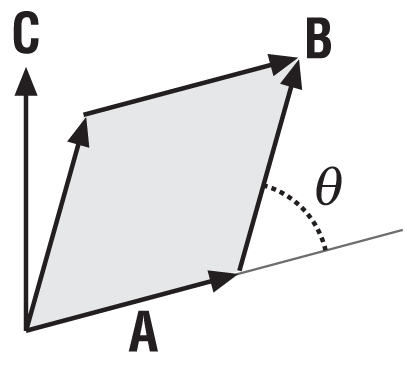
| C = A × B |
| C = AB sin θ |
The direction of C is determined by the right hand rule. As noted previously, the right hand rule is a simple trick to help you keep track of vector directions. Assume that A and B lie in a plane and let an axis of rotation extend perpendicular to this plane through a point located at the tail of A. Pretend to curl the fingers of your right hand around the axis of rotation from vector A toward B. Now extend your thumb (as though you are giving a thumbs up) while keeping your fingers curled around the axis. The direction that your thumb is pointing indicates the direction of vector C.
In the preceding figure, a parallelogram is formed by A and B (the shaded region). The area of this parallelogram is the magnitude of C, which is AB sin θ.
There are two equations that you’ll need in order to determine the vectors for tangential and centripetal acceleration. They are:
| an = ω × (ω × r) |
| at = α × r |
Another way to look at the quantities v, an, and at is that they are the velocity and acceleration of the particle under consideration, on the rigid body, relative to the point about which the rigid body is rotating—for example, the body’s center-of-mass location. This is very convenient because, as we said earlier, you’ll want to track the motion of the rigid body as a particle when viewing the big picture without having to worry about what each particle making up the rigid body is doing all the time. Thus, you treat the rigid body’s linear motion and its angular motion separately. When you do need to take a close look at specific particles of—or points on—the rigid body, you can do so by taking the motion of the rigid body as a particle and then adding to it the relative motion of the point under consideration.
Figure 2-12 shows a rigid body that is traveling at a speed vcg, where vcg is the speed of the rigid body’s center of mass (or center of gravity). Remember, the center of mass is the point to track when treating a rigid body as a particle. This rigid body is also rotating with an angular velocity ω about an axis that passes through the body’s center of mass. The vector r is the vector from the rigid body’s center of mass to the particular point of interest, P, located on the rigid body.
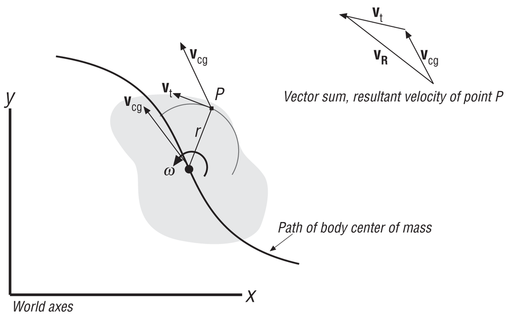
In this case, we can find the resultant velocity of the point, P, by taking the vector sum of the velocity of the body’s center of mass and the tangential velocity of point P due to the body’s angular velocity ω. Here’s what the vector equation looks like:
| vR = vcg + vt |
or:
| vR = vcg + (ω × r) |
You can do the same thing with acceleration to determine point P’s resultant acceleration. Here you’ll take the vector sum of the acceleration of the rigid body’s center of mass, the tangential acceleration due to the body’s angular acceleration, and the centripetal acceleration due to the change in direction of the tangential velocity. In equation form, this looks like:
| aR = acg + an + at |
Figure 2-13 illustrates what’s happening here.
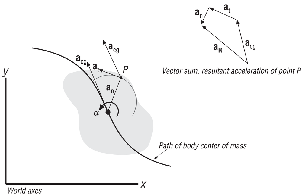
You can rewrite the equation for the resultant acceleration in the following form:
| aR = acg + (ω × (ω × r)) + (α × r) |
As you can see, using these principles of relative velocity and acceleration allows you to calculate the resultant kinematic properties of any point on a rigid body at any given time by determining what the body’s center of mass is doing along with how the body is rotating.