
Protecting Data
WORKBOOKS ARE MADE to be shared, and thus, Excel provides lots of ways in which you can easily do that. For example, you can share a workbook and track the individual changes everyone makes to it. You can later review those changes and accept or reject them as you want. See Chapter 14, “Collaborating with Others,” for help. Another way that you can protect data is to simply lock it down, preventing anyone from changing it. You can lock down individual cells, a range of cells, or an entire worksheet in order to prevent anyone from changing its data. You can also protect a whole workbook, in order to prevent changes to its structure, such as adding worksheets or changing the workbook window’s size. Finally, when needed, you can prevent unauthorized users from even opening a workbook at all.
Locking and Unlocking Cells
If your goal is to allow others to view data but to prevent them from messing it up by changing it, you must start by designating the cells you want to protect. You designate cells for protection by locking them down. After locking down cells, you turn on protection, which tells Excel to protect the data in all the locked cells. You can protect individual cells, ranges, or an entire worksheet in this way. You can also tell Excel to hide formulas. The formula result will still be shown, but not the formula itself—in other words, if someone clicks the cell, the formula is not displayed in the Formula bar.
By default, all cells in a worksheet are locked, which means that if you just turn on protection, no one will be able to change anything in the protected area. So you actually work kind of backwards, unlocking the cells you do not want to protect, and then turning on protection. Before you turn on protection, you can also hide formulas. Follow these steps to unlock the cells in a worksheet that you want to allow users to change, and to hide formulas as desired:
1. | Select the cell or range you want to unlock. |
2. | Click the Format button on the Home tab and select Lock Cell from the pop-up menu to turn that option off. |
3. | Repeat Steps 1 and 2 to unlock as many cells as you want. |
4. | To hide a formula, click its result cell, and then click the Format button on the Home tab. |
5. | Select Format Cells from the pop-up menu. The Format Cells dialog box appears. |
6. | Click the Protection tab. |
7. | Select the Hidden checkbox and click OK. |
8. | Repeat Steps 4–7 to hide additional formulas. After hiding formulas and unlocking cells, you are ready to protect the data you’ve kept locked. To protect the locked cells, you must now turn on worksheet protection. |
Tip
By default, objects are also locked when a worksheet is protected, but if you want to allow changes, you can. For example, to unlock a chart, click the chart and click the Format Selection button on the Format tab. The Format Chart Area dialog box appears; select Properties from the list on the left, deselect the Locked checkbox and click Close.
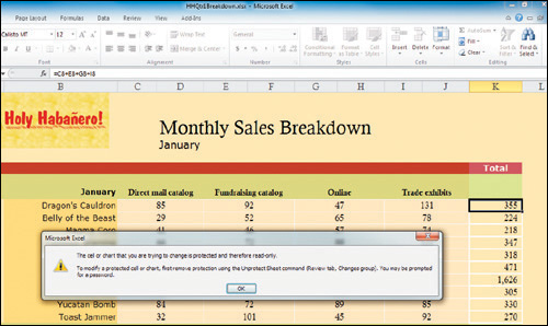
After locking cells and protecting a worksheet, users can view the data in locked cells, but not change it. If a user tries to change the data in a locked cell, a message pops up, indicating that the cell data is protected. (See Figure 13-6.) To avoid seeing a bunch of error messages, users can easily move from unlocked cell to unlocked cell by pressing Tab. By the way, a user can copy the data in locked cells, but he/she can’t move it or delete it. In addition, data can’t be copied over the top of the data in locked cells. If you’ve hidden formulas, then they disappear after your protect the worksheet (but not the formula results).
Figure 13-6. If a user attempts to change data in a cell that’s locked, a warning message appears.
Unlocking Cells with FormulasIf you unlock a cell that contains a formula, an Error Options button appears next to the cell. It serves as a reminder that you might not want to allow other people to change your formulas. However, you can click the Error Options button and select Ignore Error to turn off the warning or Lock Cell to lock the formula cell. |
Protecting a Worksheet
After unlocking the cells or objects you do not need to protect from changes, and indicating which formulas you want to hide, it’s time to turn on worksheet protection so Excel can prevent data changes to the locked cells. Follow these steps:
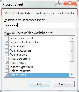
1. | Click the Format button on the Home tab and select Protect Sheet. You can also click the Protect Sheet button on the Review tab. The Protect Sheet dialog box appears, as shown in Figure 13-7. Figure 13-7. Set options for the protected sheet.
| |
2. | ||
3. | In the Allow All Users of This Worksheet To section, select the options you want to allow:
| |
4. | Click OK. | |
5. | If you entered a password in Step 2, the Confirm Password dialog box appears and you’re prompted to confirm the password by retyping it. Do so and click OK. The worksheet is immediately protected. You can repeat this process with other sheets if you want. |
After protecting a worksheet, you may find it difficult to make all the changes that you, its creator, need to make. To remove worksheet protection, click the Format button on the Home tab and select Unprotect Sheet. You can also click the Unprotect Sheet button on the Review tab. If you password-protected the sheet, type your password in the dialog box that appears and click OK. The worksheet is no longer protected.
Protecting a Workbook
In addition to protecting worksheets from unauthorized changes, you can protect entire workbooks as well. When you protect a workbook in this manner, you protect its structure—preventing users from adding, deleting, hiding, or unhiding worksheets. You can also prevent users from resizing the workbook window. Here’s how:
1. | Click the Protect Workbook button on the Review tab. The Protect Structure and Windows dialog box appears, as seen in Figure 13-8. Figure 13-8. Set options for the protected workbook.
|
2. | Select the changes you want to prevent:
|
3. | To prevent unauthorized users from unprotecting the sheet, type a password in the Password box. Passwords are case-sensitive. |
4. | Click OK. |
5. | If you entered a password in Step 3, the Confirm Password dialog box appears and you’re prompted to confirm the password by retyping it. Do so and click OK. The workbook is immediately protected. |

If you decide at some later date to remove the workbook protections (the workbook will no longer be shared, for example), just click the Protect Workbook button on the Review tab, enter the password if any, and click OK.
Preventing a Workbook from Being Opened
When the ultimate protection is needed, you can add a password to a workbook that prevents it from being opened by anyone who doesn’t know the password. Follow these steps:
1. | Click the File tab to display Backstage. |
2. | Select Info from the list on the left to display the Information options on the right. |
3. | Click the Protect Workbook button and select Encrypt With Password from the pop-up menu. The Encrypt Document dialog box appears. (See Figure 13-9.) Figure 13-9. Protect your workbook with a password.
|
4. | |
5. | Click OK. |
6. | The Confirm Password dialog box appears and you’re prompted to confirm the password by retyping it. Type the same password you typed in Step 4 and click OK. |
7. | Save the workbook to save your changes. |

Tip
Make sure you remember this password because without it, you will not be able to open the file again.
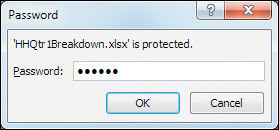
The workbook remains open so you can continue to work on it. However, after you close it, when you open it again, you are prompted to enter your password, as shown in Figure 13-10. Do so and click OK. The workbook is opened and unless other protections are in place, you can make any changes you want.
Figure 13-10. You must enter a password to view this workbook.
Removing a PasswordTo remove a password from a workbook, after opening it, follow these same steps to open the Encrypt Document dialog box. Select the password and delete it, and then click OK. Save the workbook to save your changes. |