
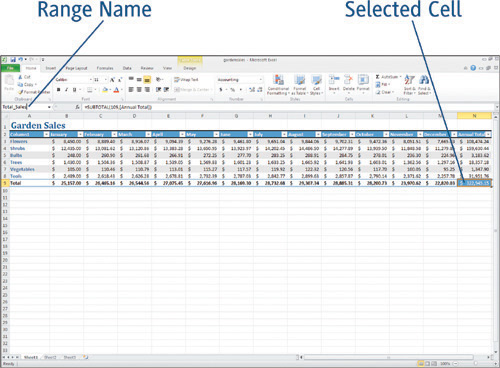
Working with Range Names
THE LARGER AND MORE COMPLEX your spreadsheets become, the harder it is to remember where the most important data is in the file. If you find yourself searching for the same data again and again, consider assigning a range name to the cells containing that data. By assigning a descriptive name to a single cell or range of cells, you will be able to find that data more quickly.
Naming a Range of Cells
Even though range names are meant to be customized to your requirements, you will still need to follow these simple rules.
Range names cannot contain spaces. Use an underscore to take the place of a space. For example, instead of Spring Sales, the range name would be Spring_Sales.
Range names must begin with a letter, not a number. For example, use Quarter_3, not 3rd_Quarter.
Range names cannot be named anything that might be interpreted by Excel to mean an actual cell address. For example, Q3 is not a good range name because it could be a valid cell address, whereas Quarter3 would make an acceptable range name.
Shorter Names Are BetterAlthough range names can be up to 255 characters long, shorter names are better as long as they are still descriptive enough to be understood. |
To name a cell or cell range, follow these steps:
1. | Select the cell or cell range you want to name. |
2. | |
3. | Press Enter to accept the change and continue working. |
Finding Named Ranges
Excel provides two methods for finding your named ranges in the spreadsheet:
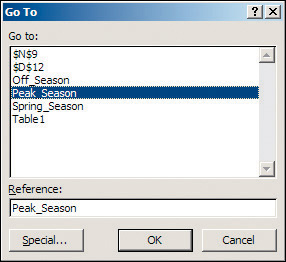
Choose Home > Editing > Find & Select > Go To and select your desired name from the list in the Go To dialog box (see Figure 1-25).
Figure 1-25. Using the Go To command to find a named range.
Click the down arrow in the Name box of the worksheet and select your desired name from the list.
In either case, Excel immediately highlights the selected cells, just as if you had selected them manually.
Using the Name Manager
You’ve learned how to add new named ranges using the Name box of your spreadsheet, but Excel also provides a Name Manager feature from the Ribbon. This tool offers you a way to edit and delete existing named ranges, as well as create new ones.
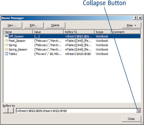
To edit or delete an existing name, choose Formulas > Defined Names > Name Manager from the Ribbon. Excel will display the Name Manager dialog box shown in Figure 1-26. Select the range name that you want to edit or delete and click the appropriate button.
To add a new name using the Name Manager:
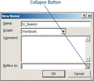
1. | Click the New button and enter a range name in the Name box. |
2. | Click the Collapse button, shown in Figure 1-27, and use your mouse to select the cells in your range. Figure 1-27. Adding a new range name using the Name Manager.
|
3. | Click the Collapse button again to return to the full-sized New Name dialog box and click OK when you are finished. |
Understanding Data Validation
YOUR WORKSHEET WORKS FOR YOU only if the data entered is valuable. Typos and carelessness can ruin your data. Imagine that you were paid solely on commission and the payroll manager made a mistake when she entered your largest sale of the year. Your wallet would be directly affected by a data entry error.
Excel provides a Data Validation feature that can help protect the data in your worksheet. Data validation helps restrict the kind of data that is entered into a specific cell, or range of cells. Data can be restricted in the following ways:
Values: You can specify that whole numbers or decimals be used, and you can choose minimum and maximum values. For instance, a realtor’s commission may be restricted to a maximum of .07, or 7%, of the sales price.
Dates and Times: You can require a specific date, or specify that the dates fall within a certain range. For example, only dates within the current year are valid.
Text: You can specify that the data in these fields is a specific length. For example, telephone numbers are 10 digits long if you include the area code and do not include the dashes.
Lists: You can create a list in another area of the worksheet and then require that all entries in the validated cell be one of the items in that list.
Accepting Blank CellsIn addition to these validation options, you can also decide whether to accept blank cells in your data. Click to deselect the Ignore Blank option when you are creating your validation to prevent your spreadsheet users from leaving blanks in the data. |
Applying Data Validation
Follow these steps to apply data validation to a range of cells:
1. | Select the cells you want Excel to validate. | ||||||||
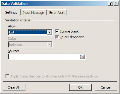
2. | Choose Data > Data Tools > Data Validation to open the Data Validation dialog box as shown in Figure 1-28. Figure 1-28. The Data Validation dialog box has three tabs.
| ||||||||
3. | |||||||||
4. | If needed, open the Data drop-down menu to refine your validation criteria. If you entered criteria in the Data box, you may also need to specify the requirements in the Minimum and Maximum boxes. | ||||||||
5. | If you choose List in the Allow drop-down menu, you have the option of entering all of the values for the list in a named range somewhere else in your spreadsheet. Make sure the In-cell drop-down option on the Settings tab is checked so that Excel will display the list of acceptable data entry items in the cell when users select that cell. | ||||||||
6. | Consider adding a message to alert users of the data validation requirements before they begin entering data. On the Input Message tab, type a message title in the Title box and type your message in the Input Message box. The users will see a pop-up message with a bold text title, shown in Figure 1-29, as soon as the cell has been selected. | ||||||||
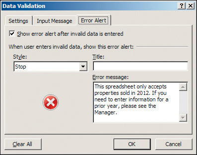
7. | Excel displays a default error message when data entered into a cell cannot be validated. You can specify the text on the message to remind users exactly what the rules are for a particular cell. From the Error Alert tab (see Figure 1-30), type a title for the message in the Title box, and type your message in the Error Message box. Figure 1-30. The Error Alert tab on the Data Validation dialog box.
| ||||||||
8. | Choose one of the following error message styles from the Style drop-down menu.
| ||||||||
9. | Click OK to close the Data Validation dialog box. |

Removing Data ValidationTo remove data validation from a selected cell or cell range, choose Data > Data Tools > Data Validation. Click the Clear All button in the Data Validation dialog box and click OK to accept the change. |
Using Data Validation
Excel provides two other useful data validation features. The first shows you all of the cells in your spreadsheet that have validation restrictions. The second shows you all of the cells that contain invalid data.
Choose Home > Editing > Find & Select > Data Validation. All cells with any kind of validation restrictions will be highlighted, as if you had selected them with the mouse.
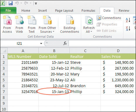
Choose Data > Data Tools > Data Validation (arrow). Choose Circle Invalid Data. Excel will place a red circle (see Figure 1-31) around any cells that contain invalid data. Choose Data Validation (arrow) and then Clear Validation Circles to remove the red circles.
Figure 1-31. Excel shows you which cells contain validation errors.
Saving a Worksheet
PICTURE YOURSELF WORKING for hours to create the perfect worksheet and then your neighborhood or office complex suffers a power outage and all of your hard work is lost. Well, that might have happened in the past, but Excel has gone a long way to dispel that disheartening experience with its AutoSave feature. Every 10 minutes, Excel will save a copy of your file. In this way, even in the event of a power failure, you can be sure that you will never lose more than 10 minutes’ worth of work.
But don’t rely solely on the AutoSave feature. Get into the habit of saving your file shortly after you begin working on it. You will be able to replace the temporary Book1 file name with a more descriptive name and store the file in an appropriate location on your computer or network.
Tip
If you need to share your file with friends who have not yet upgraded to Excel 2010, you should change the file type. Click the Save As Type down arrow and select Excel 97-2003 Workbook. Other options for sharing your files are discussed in Chapter 14, “Collaborating with Others.”
Saving the First Time
The first time you save your file, choose File > Save As from the Ribbon. Excel displays the Save As dialog box, as shown in Figure 1-32. From the Save As dialog box, enter the following information about your document.
File name: Feel free to be as descriptive as you want, within reason. You have 255 characters, including spaces, to name your files.
Location: Use the Save In folder or the favorite links area to find the perfect location in which to store this file.
Save As Type: Excel Workbook, as shown in Figure 1-32, is the default file type in Excel 2010 files.
Adding the following information about your file is optional. However, Excel stores this data with your document so that you can use any or all of it if you need to use the Search box to find a file you misplaced.
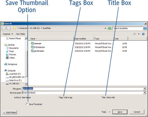
Save Thumbnail: Select this option and Excel will store a thumbnail image, or miniature picture, of your file next to the file name. In this way, the thumbnail acts as a preview of your file to help you recognize it when you are ready to re-open the file (see Figure 1-33).
Figure 1-33. A thumbnail image of your file appears next to the file name in the folders.
Tags: Click the Tags box to add any words that you might associate with your file. For instance, a spreadsheet to track the family budget might include the tag “budget” or “financial”.
Title: Click the Title box to add a title. This might be important if you used abbreviations in your file name. Suppose your file name was FY2012. You might choose to add Fiscal Year 2012 to the Title box.
Tip
You will only need to use the File > Save As command once. Once you have specified the file name and location that you want associated with your document, you can press Ctrl+S, or choose File > Save from the Ribbon, to save a copy of your document at any time. However, use the File > Save As command again any time you need to move or rename the file.
Closing and Exiting Excel
When you are ready to stop work for the day, there are several ways to exit an Office application.
Choose File > Exit from the Ribbon.
Choose Alt+F4 from the keyboard.
Click the Close button in the upper-right corner of the Excel application window.
Click the Excel program icon > Close command in the upper-left corner of the Excel application window.