
Creating an AutoFilter
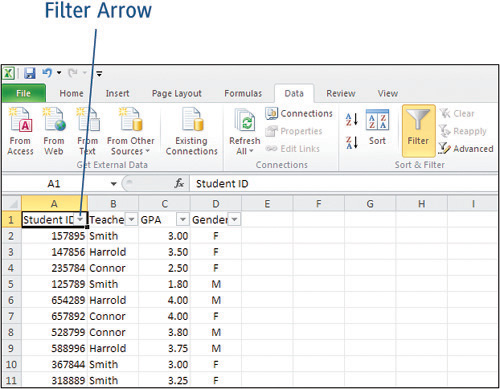
THE EASIEST WAY TO FILTER your data is to use the AutoFilter feature in Excel. To create an AutoFilter, click anywhere in your worksheet table and choose Data > Sort & Filter > Filter. Excel recognizes that all of the adjacent cells are part of your table and applies a filter arrow to the top cell in each column, as seen in Figure 8-1.
Figure 8-1. The AutoFilter feature applies a filter arrow to each column in your worksheet’s table.
Caution

| The AutoFilter feature does not work on protected worksheets. Learn more about protecting worksheets in Chapter 13, “Setting Security Options.” |
Applying the Filters
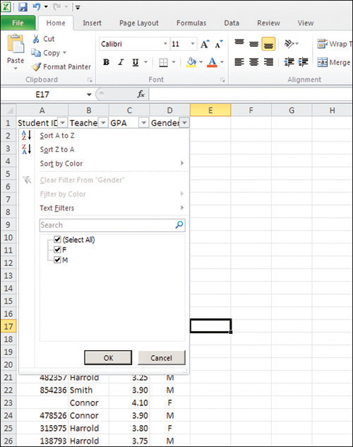
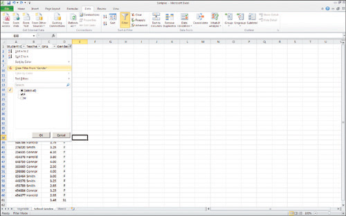
Clicking the filter arrow in each column header displays a drop-down menu of the unique entries in that column. In Figure 8-2, you can see that the unique values in the Gender column are F and M.
To apply a filter to your data, follow these steps.
Tip
The AutoFilter’s drop-down menu will show up to 10,000 unique data points, such as product numbers. You may need to use additional criteria to filter some of your tables.
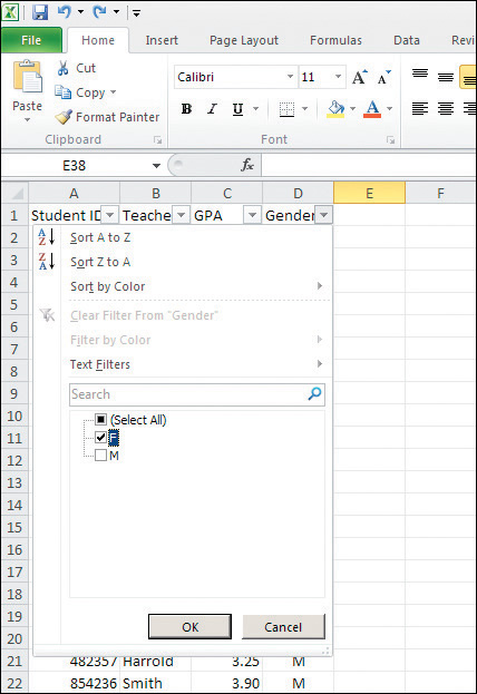
1. | Remove the check mark from the Select All option. The check marks are automatically removed from the rest of the unique entries. |
2. | Click the filtering option you want to see on your worksheet and click OK to apply the filter. In Figure 8-3, selecting the F option from the Gender column will filter out any records with an M in that column. Figure 8-3. Select only those values you want to see in your filtered worksheet data.
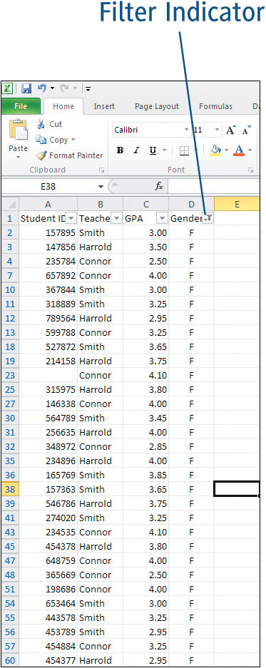
The correct filtered data is displayed in the worksheet and the filter arrow has changed (see Figure 8-4). Once a filter is applied, the image next to the column title changes to look like a funnel to indicate that a filter is in use. Figure 8-4. The arrow on the column header becomes a funnel once a filter has been applied.
|
To remove the filters from the worksheet and return to the full unfiltered list of data, choose one of the following options:
Click the filter button next to the column header and choose Clear Filter (see Figure 8-5).
Click the Select All option and then click OK.
Choose Data > Filter from the Ribbon.
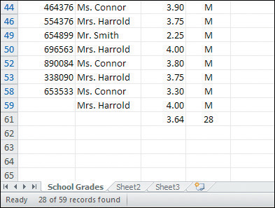
Number of Records DisplayedWhenever a filter is applied to your data, the number of records displayed appears in Excel’s status bar. In Figure 8-6, Excel found that 28 of the 59 records in the worksheet database fit the filter. Figure 8-6. The status bar displays the number of records matching your filter.
|
Copying Filtered Data
After you have filtered your data to display only the files relevant to your needs, you can copy that data to the Microsoft Clipboard. From the Clipboard, you can paste the filtered data into another area of your worksheet, or into any other Microsoft application.
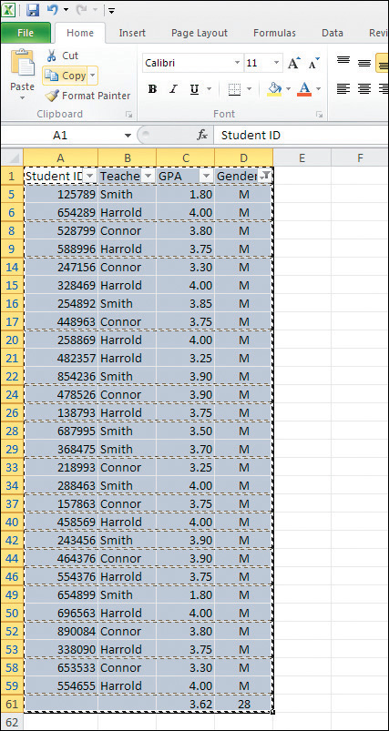
Use your mouse to select the filtered data and choose Home > Copy to copy the data to the Clipboard. Look closely at the highlighted cells in Figure 8-7. Excel automatically performs a non-adjacent cell selection to copy only the filtered data. Notice that the marquee, or the marching ants, appears between filtered data cells.
Figure 8-7. Excel copies only filtered data to the Clipboard.
Choose one of the following options to paste your data.
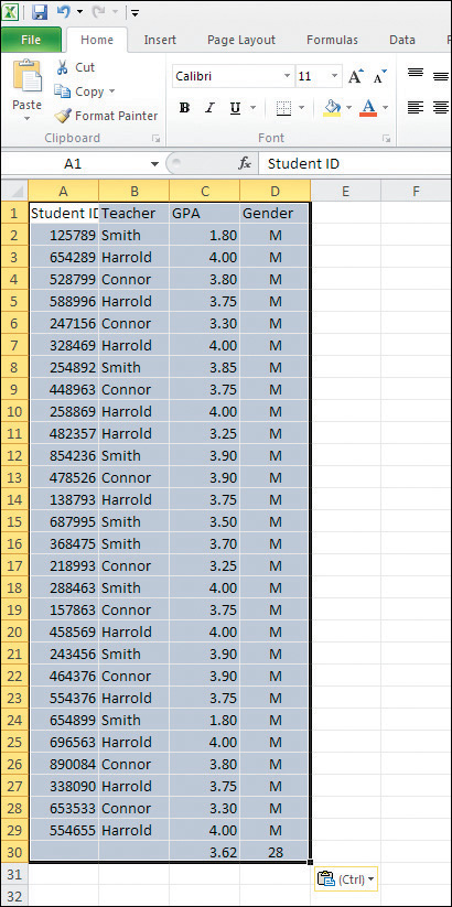
To paste your data into a new Excel worksheet, or into another area of the existing worksheet, select the first cell in the destination worksheet and choose Home > Paste. Once pasted into the new area of the worksheet, the new data is formatted as an unfiltered table. Take a closer look at the row numbers displayed in Figure 8-8; the data hidden in the original area of the filtered worksheet table has now been permanently removed.
Figure 8-8. Excel deletes everything but the filtered data when you paste filtered data.
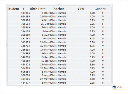
To paste your data into another Microsoft application, open the new application and position your cursor where desired, then press Ctrl+V to paste your data into the application. Figure 8-9 illustrates how your data will appear when pasted into PowerPoint 2010.
Tip
Once the data has been pasted into the new application, it can be formatted using the application’s standard formatting tools, as shown in Figure 8-10.

Filter Arrows Aren’t CopiedThe filter arrows are overlaid onto your worksheet; they are not part of your worksheet. As such, they will not be copied with your data. |