Chapter 10: Performance and Concurrency
Performance and concurrency are two problems that are often tightly coupled—when concurrency problems are encountered, performance usually degrades, in some cases by a lot. If you take care of concurrency problems, you will achieve better performance.
In this chapter, you will see how to find slow queries and how to find queries that make other queries slow.
Performance tuning, unfortunately, is still not an exact science, so you may also encounter a performance problem that's not covered by any of the given methods.
We will also see how to get help in the final recipe, Reporting performance problems, in case none of the other recipes that are covered here work.
In this chapter, we will cover the following recipes:
- Finding slow SQL statements
- Finding out what makes SQL slow
- Reducing the number of rows returned
- Simplifying complex SQL queries
- Speeding up queries without rewriting them
- Discovering why a query is not using an index
- Forcing a query to use an index
- Using parallel query
- Creating time-series tables using partitioning
- Using optimistic locking to avoid long lock waits
- Reporting performance problems
Finding slow SQL statements
Two main kinds of slowness can manifest themselves in a database.
The first kind is a single query that can be too slow to be really usable, such as a customer information query in a customer relationship management (CRM) system running for minutes, a password check query running in tens of seconds, or a daily data aggregation query running for more than a day. These can be found by logging queries that take over a certain amount of time, either at the client end or in the database.
The second kind is a query that is run frequently (say a few thousand times a second) and used to run in single-digit milliseconds (ms) but is now running in several tens or even hundreds of milliseconds, hence slowing the system down.
Here, we will show you several ways to find statements that are either slow or cause the database as a whole to slow down (although they are not slow by themselves).
Getting ready
Connect to the database as the user whose statements you want to investigate or as a superuser to investigate all users' querie:.
- Check that you have the pg_stat_statements extension installed:
postgres=# x
postgres=# dx pg_stat_statements
- Here is a list of our installed extensions:
-[ RECORD 1 ]-------------------------------------------------------
Name | pg_stat_statements
Version | 1.9
Schema | public
Description | track execution statistics of all SQL statements executed
- If you can't see them, then issue the following command:
postgres=# CREATE EXTENSION pg_stat_statements;
postgres=# ALTER SYSTEM
SET shared_preload_libraries = 'pg_stat_statements';
- Then, restart the server, or refer to the Using an installed module and Managing installed extensions recipes from Chapter 3, Server Configuration, for more details.
How to do it…
Run this query to look at the top 10 highest workloads on your server side:
postgres=# SELECT calls, total_exec_time, query
FROM pg_stat_statements
ORDER BY total_exec_time DESC LIMIT 10;
The output is ordered by total_exec_time, so it doesn't matter whether it was a single query or thousands of smaller queries.
Many additional columns are useful in tracking down further information about particular entries:
postgres=# d pg_stat_statements
View "public.pg_stat_statements"
Column | Type | Modifiers
---------------------+------------------+-----------
userid | oid |
dbid | oid |
toplevel | bool |
Unique identifier for SQL
queryid | bigint |
The SQL being executed
query | text |
Number of times planned and timings
plans | bigint |
total_plan_time | double precision |
min_plan_time | double precision |
max_plan_time | double precision |
mean_plan_time | double precision |
stddev_plan_time | double precision |
Number of times executed and timings
calls | bigint |
total_exec_time | double precision |
min_exec_time | double precision |
max_exec_time | double precision |
mean_exec_time | double precision |
stddev_exec_time | double precision |
Number of rows returned by query
rows | bigint |
Columns related to tables that all users can access
shared_blks_hit | bigint |
shared_blks_read | bigint |
shared_blks_dirtied | bigint |
shared_blks_written | bigint |
Columns related to session-specific temporary tables
local_blks_hit | bigint |
local_blks_read | bigint |
local_blks_dirtied | bigint |
local_blks_written | bigint |
Columns related to temporary files
temp_blks_read | bigint |
temp_blks_written | bigint |
I/O timing
blk_read_time | double precision |
blk_write_time | double precision |
Columns related to WAL usage
wal_records | bigint |
wal_fpi | bigint |
wal_bytes | numeric |
How it works…
pg_stat_statements collects data on all running queries by accumulating data in memory, with low overheads.
Similar SQL statements are normalized so that the constants and parameters that are used for execution are removed. This allows you to see all similar SQL statements in one line of the report, rather than seeing thousands of lines, which would be fairly useless. While useful, it can sometimes mean that it's hard to work out which parameter values are actually causing the problem.
There's more…
Another way to find slow queries is to set up PostgreSQL to log them to the server log. For example, if you decide to monitor any query that takes over 10 seconds, then use the following command:
postgres=# ALTER SYSTEM
SET log_min_duration_statement = 10000;
Remember that the duration is in ms. After doing this, reload PostgreSQL. All queries whose duration exceeds the threshold will be logged. You should pick a threshold that is above 99% of queries so that you only get the worst outliers logged. As you progressively tune your system, you can reduce the threshold over time.
PostgreSQL log files are usually located together with other log files; for example, on Debian/Ubuntu Linux, they are in the /var/log/postgresql/ directory.
If you set log_min_duration_statement = 0, then all queries would be logged, which will typically swamp the log file, causing more performance problems itself, and thus this is not recommended. A better idea would be to use the log_min_duration_sample parameter, available in PostgreSQL 13+, to set a limit for sampling queries. The two settings are designed to work together:
- Any query elapsed time less than log_min_duration_sample is not logged at all.
- Any query elapsed time higher than log_min_duration_statement is always logged.
- For any query elapsed time that falls between the two settings, we sample the queries and log them at a rate set by log_statement_sample_rate (default 1.0 = all). Note that the sampling is blind—it is not stratified/weighted, so rare queries may not show up at all in the log.
Query logging will show the parameters that are being used for the slow query, even when pg_stat_statements does not.
Finding out what makes SQL slow
An SQL statement can be slow for a lot of reasons. Here, we will provide a short list of these reasons, with at least one way of recognizing each.
Getting ready
If the SQL statement is still running, look at Chapter 8, Monitoring and Diagnosis.
How to do it…
The core issues are likely to be the following:
- You're asking the SQL statement to do too much work.
- Something is stopping the SQL statement from doing the work.
This might not sound that helpful at first, but it's good to know that there's nothing really magical going on that you can't understand if you look.
In more detail, the main reasons/issues are these:
- Returning too much data.
- Processing too much data.
- Index needed.
- The wrong plan for other reasons—for example, poor estimates.
- Locking problems.
- Cache or input/output (I/O) problems. It's possible the system itself has bottlenecks such as single-core, slow central processing units (CPUs), insufficient memory, or reduced I/O throughput. Those issues may be outside the scope of this book—here, we discuss just the database issues.
The first issue can be handled as described in the Reducing the number of rows returned recipe. The rest of the preceding reasons can be investigated from two perspectives: the SQL itself and the objects that the SQL touches. Let's start by looking at the SQL itself by running the query with EXPLAIN ANALYZE. We're going to use the optional form, as follows:
postgres=# EXPLAIN (ANALYZE, BUFFERS) ...SQL...
The EXPLAIN command provides output to describe the execution plan of the SQL, showing access paths and costs (in abstract units). The ANALYZE option causes the statement to be executed (be careful), with instrumentation to show the number of rows accessed and the timings for that part of the plan. The BUFFERS option provides information about the number of database buffers read and the number of buffers that were hit in the cache. Taken together, we have everything we need to diagnose whether the SQL performance is reduced by one of the earlier mentioned issues:
postgres=# EXPLAIN (ANALYZE, BUFFERS) SELECT count(*) FROM t;
QUERY PLAN
--------------------------------------------------------------
Aggregate (cost=4427.27..4427.28 rows=1 width=0)
(actual time=32.953..32.954 rows=1 loops=1)
Buffers: shared hit=X read=Y
-> Seq Scan on t (cost=0.00..4425.01 rows=901 width=0)
(actual time=30.350..31.646 rows=901 loops=1)
Buffers: shared hit=X read=Y
Planning time: 0.045 ms
Execution time: 33.128 ms
(6 rows)
Let's use this technique to look at an SQL statement that would benefit from an index.
For example, if you want to get the three latest rows in a 1 million row table, run the following query:
SELECT * FROM events ORDER BY id DESC LIMIT 3;
You can either read through just three rows using an index on the id SERIAL column or you can perform a sequential scan of all rows followed by a sort, as shown in the following code snippet. Your choice depends on whether you have a usable index on the field from which you want to get the top three rows:
postgres=# CREATE TABLE events(id SERIAL);
CREATE TABLE
postgres=# INSERT INTO events SELECT generate_series(1,1000000);
INSERT 0 1000000
postgres=# EXPLAIN (ANALYZE)
SELECT * FROM events ORDER BY id DESC LIMIT 3;
QUERY PLAN
--------------------------------------------------------------
Limit (cost=25500.67..25500.68 rows=3 width=4)
(actual time=3143.493..3143.502 rows=3 loops=1)
-> Sort (cost=25500.67..27853.87 rows=941280 width=4)
(actual time=3143.488..3143.490 rows=3 loops=1)
Sort Key: id DESC
Sort Method: top-N heapsort Memory: 25kB
-> Seq Scan on events
(cost=0.00..13334.80 rows=941280 width=4)
(actual time=0.105..1534.418 rows=1000000 loops=1)
Planning time: 0.331 ms
Execution time: 3143.584 ms
(10 rows)
postgres=# CREATE INDEX events_id_ndx ON events(id);
CREATE INDEX
postgres=# EXPLAIN (ANALYZE)
SELECT * FROM events ORDER BY id DESC LIMIT 3;
QUERY PLAN
--------------------------------------------------------------------
Limit (cost=0.00..0.08 rows=3 width=4) (actual
time=0.295..0.311 rows=3 loops=1)
-> Index Scan Backward using events_id_ndx on events
(cost=0.00..27717.34 rows=1000000 width=4) (actual
time=0.289..0.295 rows=3 loops=1)
Total runtime: 0.364 ms
(3 rows)
This produces a huge difference in query runtime, even when all of the data is in the cache.
If you run the same analysis using EXPLAIN (ANALYZE, BUFFERS) on your production system, you'll be able to see the cache effects as well. Databases work well if the "active set" of data blocks in a database can be cached in random-access memory (RAM). The active set, also known as the working set, is a subset of the data that is accessed by queries on a regular basis. Each new index you add will increase the pressure on the cache, so it is possible to have too many indexes.
You can also look at the statistics for objects touched by queries, as mentioned in the Knowing whether anybody is using a specific table recipe from Chapter 8, Monitoring and Diagnosis. In pg_stat_user_tables, the fast growth of seq_tup_read means that there are lots of sequential scans occurring. The ratio of seq_tup_read to seq_scan shows how many tuples each seqscan reads. Similarly, the idx_scan and idx_tup_fetch columns show whether indexes are being used and how effective they are.
There's more…
If not enough of the data fits in the shared buffers, lots of rereading of the same data happens, causing performance issues. In pg_statio_user_tables, watch the heap_blks_hit and heap_blks_read fields, or the equivalent ones for index and toast relations. They give you a fairly good idea of how much of your data is found in PostgreSQL's shared buffers (heap_blks_hit) and how much had to be fetched from the disk (heap_blks_read). If you see large numbers of blocks being read from the disk continuously, you may want to tune those queries; if you determine that the disk reads were justified, you can make the configured shared_buffers value bigger.
If your shared_buffers parameter is tuned properly and you can't rewrite the query to perform less block I/O, you might need a bigger server.
You can find a lot of resources on the web that explain how shared buffers work and how to set them based on your available hardware and your expected data access patterns. Our professional advice is to always test your database servers and perform benchmarks before you deploy them in production. Information on the shared_buffers configuration parameter can be found at http://www.postgresql.org/docs/current/static/runtime-config-resource.html.
Locking problems
Thanks to its multi-version concurrency control (MVCC) design, PostgreSQL does not suffer from most locking problems, such as writers locking out readers or readers locking out writers, but it still has to take locks when more than one process wants to update the same row. Also, it has to hold the write lock until the current writer's transaction finishes.
So, if you have a database design where many queries update the same record, you can have a locking problem. Running Data Definition Language (DDL) will also require stronger locks that may interrupt applications.
Refer to the Knowing who is blocking a query recipe of Chapter 8, Monitoring and Diagnosis, for more detailed information.
To diagnose locking problems retrospectively, use the log_lock_waits parameter to generate log output for locks that are held for a long time.
EXPLAIN options
Use the FORMAT option to retrieve the output of EXPLAIN in a different format, such as JavaScript Object Notation (JSON), Extensible Markup Language (XML), and YAML Ain't Markup Language (YAML). This could allow us to write programs to manipulate the outputs.
The following command is an example of this:
EXPLAIN (ANALYZE, BUFFERS, FORMAT JSON) SELECT count(*) FROM t;
Not enough CPU power or disk I/O capacity for the current load
These issues are usually caused by suboptimal query plans but, sometimes, your computer is just not powerful enough.
In this case, top is your friend. For quick checks, run the following code from the command line:
user@host:~$ top
First, watch the percentage of idle CPU from top. If this is in low single digits most of the time, you probably have problems with the CPU's power.
If you have a high load average with a lot of CPU idle left, you are probably out of disk bandwidth. In this case, you should also have lots of Postgres processes in the D status, meaning that the process is in an uninterruptible state (usually waiting for I/O).
See also
For further information on the syntax of the EXPLAIN SQL command, refer to the PostgreSQL documentation at http://www.postgresql.org/docs/current/static/sql-explain.html.
Reducing the number of rows returned
Although the problem often produces too many rows in the first place, it is made worse by returning all unnecessary rows to the client. This is especially true if the client and server are not on the same host.
Here are some ways to reduce the traffic between the client and server.
How to do it…
Consider the following scenario: a full-text search returns 10,000 documents, but only the first 20 are displayed to users. In this case, order the documents by rank on the server, and return only the top 20 that actually need to be displayed:
SELECT title, ts_rank_cd(body_tsv, query, 20) AS text_rank
FROM articles, plainto_tsquery('spicy potatoes') AS query
WHERE body_tsv @@ query
ORDER BY rank DESC
LIMIT 20
;
The ORDER BY clause ensures the rows are ranked, and then the LIMIT 20 returns only the top 20.
If you need the next 20 documents, don't just query with a limit of 40 and throw away the first 20. Instead, use OFFSET 20 LIMIT 20 to return the next 20 documents.
The SQL optimizer understands the LIMIT clause and will change the execution plan accordingly.
To gain some stability so that documents with the same rank still come out in the same order when using OFFSET 20, add a unique field (such as the id column of the articles table) to ORDER BY in both queries:
SELECT title, ts_rank_cd(body_tsv, query, 20) AS text_rank
FROM articles, plainto_tsquery('spicy potatoes') AS query
WHERE body_tsv @@ query
ORDER BY rank DESC, articles.id
OFFSET 20 LIMIT 20;
Another use case is an application that requests all products of a branch office so that it can run a complex calculation over them. In such a case, try to do as much data analysis as possible inside the database.
There is no need to run the following:
SELECT * FROM accounts WHERE branch_id = 7;
Also, instead of counting and summing the rows on the client side, you can run this:
SELECT count(*), sum(balance) FROM accounts WHERE branch_id = 7;
With some research on SQL, you can carry out an amazingly large portion of your computation using plain SQL (for example, do not underestimate the power of window functions).
If SQL is not enough, you can use Procedural Language/PostgreSQL (PL/pgSQL) or any other embedded procedural language supported by PostgreSQL for even more flexibility.
There's more…
Consider one more scenario: an application runs a huge number of small lookup queries. This can easily happen with modern object-relational mappers (ORMs) and other toolkits that do a lot of work for the programmer but, at the same time, hide a lot of what is happening.
For example, if you define a HyperText Markup Language (HTML) report over a query in a templating language and then define a lookup function to resolve an identifier (ID) inside the template, you may end up with a form that performs a separate, small lookup for each row displayed, even when most of the values looked up are the same. This doesn't usually pose a big problem for the database, as queries of the SELECT name FROM departments WHERE id = 7 form are really fast when the row for id = 7 is in shared buffers. However, repeating this query thousands of times still takes seconds due to network latency, process scheduling for each request, and other factors.
The two proposed solutions are as follows:
- Make sure that the value is cached by your ORM
- Perform the lookup inside the query that gets the main data so that it can be displayed directly
Exactly how to carry out these solutions depends on the toolkit, but they are both worth investigating as they really can make a difference in speed and resource usage.
PostgreSQL 9.5 introduced the TABLESAMPLE clause into SQL. This allows you to run commands much faster by using a sample of a table's rows, giving an approximate answer. In certain cases, this can be just as useful as the most accurate answer:
postgres=# SELECT avg(id) FROM events;
avg
---------------------
500000.500
(1 row)
postgres=# SELECT avg(id) FROM events TABLESAMPLE system(1);
avg
---------------------
507434.635
(1 row)
postgres=# EXPLAIN (ANALYZE, BUFFERS) SELECT avg(id) FROM events;
QUERY PLAN
--------------------------------------------------------------------
Aggregate (cost=16925.00..16925.01 rows=1 width=32) (actual time=204.841..204.841 rows=1 loops=1)
Buffers: shared hit=96 read=4329
-> Seq Scan on events (cost=0.00..14425.00 rows=1000000 width=4) (actual time=1.272..105.452 rows=1000000 loops=1)
Buffers: shared hit=96 read=4329
Planning time: 0.059 ms
Execution time: 204.912 ms
(6 rows)
postgres=# EXPLAIN (ANALYZE, BUFFERS)
SELECT avg(id) FROM events TABLESAMPLE system(1);
QUERY PLAN
--------------------------------------------------------------------
Aggregate (cost=301.00..301.01 rows=1 width=32) (actual time=4.627..4.627 rows=1 loops=1)
Buffers: shared hit=1 read=46
-> Sample Scan on events (cost=0.00..276.00 rows=10000 width=4) (actual time=0.074..2.833 rows=10622 loops=1)
Sampling: system ('1'::real)
Buffers: shared hit=1 read=46
Planning time: 0.066 ms
Execution time: 4.702 ms
(7 rows)
Simplifying complex SQL queries
There are two types of complexity that you can encounter in SQL queries.
First, the complexity can be directly visible in the query if it has hundreds—or even thousands—of rows of SQL code in a single query. This can cause both maintenance headaches and slow execution.
This complexity can also be hidden in subviews, so the SQL code of the query may seem simple but it uses other views and/or functions to do part of the work, which can, in turn, use others. This is much better for maintenance, but it can still cause performance problems.
Both types of queries can either be written manually by programmers or data analysts or emerge as a result of a query generator.
Getting ready
First, verify that you really have a complex query.
A query that simply returns lots of database fields is not complex in itself. In order to be complex, the query has to join lots of tables in complex ways.
The easiest way to find out whether a query is complex is to look at the output of EXPLAIN. If it has lots of rows, the query is complex, and it's not just that there is a lot of text that makes it so.
All of the examples in this recipe have been written with a very typical use case in mind: sales.
What follows is a description of a fictitious model that's used in this recipe. The most important fact is the sale event, stored in the sale table (I specifically used the word fact, as this is the right term to use in a data warehousing context). Every sale takes place at a point of sale (the salespoint table) at a specific time and involves an item. That item is stored in a warehouse (see the item and warehouse tables, as well as the item_in_wh link table).
Both warehouse and salespoint are located in a geographical area (the location table). This is important, for example, to study the provenance of a transaction.
Here is a simplified entity-relationship model (ERM), which is useful for understanding all of the joins that occur in the following queries:
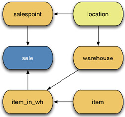
Figure 10.1 – Data model for the example code
How to do it…
Simplifying a query usually means restructuring it so that parts of it can be defined separately and then used by other parts.
We'll illustrate these possibilities by rewriting the following query in several ways.
The complex query in our example case is a so-called pivot or cross-tab query. This query retrieves the quarterly profit for non-local sales from all shops, as shown in the following code snippet:
SELECT shop.sp_name AS shop_name,
q1_nloc_profit.profit AS q1_profit,
q2_nloc_profit.profit AS q2_profit,
q3_nloc_profit.profit AS q3_profit,
q4_nloc_profit.profit AS q4_profit,
year_nloc_profit.profit AS year_profit
FROM (SELECT * FROM salespoint ORDER BY sp_name) AS shop
LEFT JOIN (
SELECT
spoint_id,
sum(sale_price) - sum(cost) AS profit,
count(*) AS nr_of_sales
FROM sale s
JOIN item_in_wh iw ON s.item_in_wh_id=iw.id
JOIN item i ON iw.item_id = i.id
JOIN salespoint sp ON s.spoint_id = sp.id
JOIN location sploc ON sp.loc_id = sploc.id
JOIN warehouse wh ON iw.whouse_id = wh.id
JOIN location whloc ON wh.loc_id = whloc.id
WHERE sale_time >= '2013-01-01'
AND sale_time < '2013-04-01'
AND sploc.id != whloc.id
GROUP BY 1
) AS q1_nloc_profit
ON shop.id = Q1_NLOC_PROFIT.spoint_id
LEFT JOIN (
< similar subquery for 2nd quarter >
) AS q2_nloc_profit
ON shop.id = q2_nloc_profit.spoint_id
LEFT JOIN (
< similar subquery for 3rd quarter >
) AS q3_nloc_profit
ON shop.id = q3_nloc_profit.spoint_id
LEFT JOIN (
< similar subquery for 4th quarter >
) AS q4_nloc_profit
ON shop.id = q4_nloc_profit.spoint_id
LEFT JOIN (
< similar subquery for full year >
) AS year_nloc_profit
ON shop.id = year_nloc_profit.spoint_id
ORDER BY 1;
Since the preceding query has an almost identical repeating part for finding the sales for a period (the four quarters of 2013, in this case), it makes sense to move it to a separate view (for the whole year) and then use that view in the main reporting query, as follows:
CREATE VIEW non_local_quarterly_profit_2013 AS
SELECT
spoint_id,
extract('quarter' from sale_time) as sale_quarter,
sum(sale_price) - sum(cost) AS profit,
count(*) AS nr_of_sales
FROM sale s
JOIN item_in_wh iw ON s.item_in_wh_id=iw.id
JOIN item i ON iw.item_id = i.id
JOIN salespoint sp ON s.spoint_id = sp.id
JOIN location sploc ON sp.loc_id = sploc.id
JOIN warehouse wh ON iw.whouse_id = wh.id
JOIN location whloc ON wh.loc_id = whloc.id
WHERE sale_time >= '2013-01-01'
AND sale_time < '2014-01-01'
AND sploc.id != whloc.id
GROUP BY 1,2;
SELECT shop.sp_name AS shop_name,
q1_nloc_profit.profit as q1_profit,
q2_nloc_profit.profit as q2_profit,
q3_nloc_profit.profit as q3_profit,
q4_nloc_profit.profit as q4_profit,
year_nloc_profit.profit as year_profit
FROM (SELECT * FROM salespoint ORDER BY sp_name) AS shop
LEFT JOIN non_local_quarterly_profit_2013 AS q1_nloc_profit
ON shop.id = Q1_NLOC_PROFIT.spoint_id
AND q1_nloc_profit.sale_quarter = 1
LEFT JOIN non_local_quarterly_profit_2013 AS q2_nloc_profit
ON shop.id = Q2_NLOC_PROFIT.spoint_id
AND q2_nloc_profit.sale_quarter = 2
LEFT JOIN non_local_quarterly_profit_2013 AS q3_nloc_profit
ON shop.id = Q3_NLOC_PROFIT.spoint_id
AND q3_nloc_profit.sale_quarter = 3
LEFT JOIN non_local_quarterly_profit_2013 AS q4_nloc_profit
ON shop.id = Q4_NLOC_PROFIT.spoint_id
AND q4_nloc_profit.sale_quarter = 4
LEFT JOIN (
SELECT spoint_id, sum(profit) AS profit
FROM non_local_quarterly_profit_2013 GROUP BY 1
) AS year_nloc_profit
ON shop.id = year_nloc_profit.spoint_id
ORDER BY 1;
Moving the subquery to a view has not only made the query shorter but also easier to understand and maintain.
You might want to consider materialized views—more on this later.
Before that, we will be using common table expressions (also known as WITH queries) instead of a separate view. Starting with PostgreSQL version 8.4, you can use a WITH statement to define a view in line, as follows:
WITH nlqp AS (
SELECT
spoint_id,
extract('quarter' from sale_time) as sale_quarter,
sum(sale_price) - sum(cost) AS profit,
count(*) AS nr_of_sales
FROM sale s
JOIN item_in_wh iw ON s.item_in_wh_id=iw.id
JOIN item i ON iw.item_id = i.id
JOIN salespoint sp ON s.spoint_id = sp.id
JOIN location sploc ON sp.loc_id = sploc.id
JOIN warehouse wh ON iw.whouse_id = wh.id
JOIN location whloc ON wh.loc_id = whloc.id
WHERE sale_time >= '2013-01-01'
AND sale_time < '2014-01-01'
AND sploc.id != whloc.id
GROUP BY 1,2
)
SELECT shop.sp_name AS shop_name,
q1_nloc_profit.profit as q1_profit,
q2_nloc_profit.profit as q2_profit,
q3_nloc_profit.profit as q3_profit,
q4_nloc_profit.profit as q4_profit,
year_nloc_profit.profit as year_profit
FROM (SELECT * FROM salespoint ORDER BY sp_name) AS shop
LEFT JOIN nlqp AS q1_nloc_profit
ON shop.id = Q1_NLOC_PROFIT.spoint_id
AND q1_nloc_profit.sale_quarter = 1
LEFT JOIN nlqp AS q2_nloc_profit
ON shop.id = Q2_NLOC_PROFIT.spoint_id
AND q2_nloc_profit.sale_quarter = 2
LEFT JOIN nlqp AS q3_nloc_profit
ON shop.id = Q3_NLOC_PROFIT.spoint_id
AND q3_nloc_profit.sale_quarter = 3
LEFT JOIN nlqp AS q4_nloc_profit
ON shop.id = Q4_NLOC_PROFIT.spoint_id
AND q4_nloc_profit.sale_quarter = 4
LEFT JOIN (
SELECT spoint_id, sum(profit) AS profit
FROM nlqp GROUP BY 1
) AS year_nloc_profit
ON shop.id = year_nloc_profit.spoint_id
ORDER BY 1;
For more information on WITH queries (also known as Common Table Expressions (CTEs)), read the official documentation at http://www.postgresql.org/docs/current/static/queries-with.html.
There's more…
Another ace in the hole is represented by temporary tables that are used for parts of a query. By default, a temporary table is dropped at the end of a Postgres session, but the behavior can be changed at the time of creation.
PostgreSQL itself can choose to materialize parts of a query during the query optimization phase but, sometimes, it fails to make the best choice for the query plan, either due to insufficient statistics or because—as can happen for large query plans where Genetic Query Optimization (GEQO) is used—it may have just overlooked some possible query plans.
If you think that materializing (separately preparing) some parts of a query is a good idea, you can do this by using a temporary table, simply by running CREATE TEMPORARY TABLE my_temptable01 AS <the part of the query you want to materialize> and then using my_temptable01 in the main query, instead of the materialized part.
You can even create indexes on a temporary table for PostgreSQL to use in the main query:
BEGIN;
CREATE TEMPORARY TABLE nlqp_temp ON COMMIT DROP
AS
SELECT
spoint_id,
extract('quarter' from sale_time) as sale_quarter,
sum(sale_price) - sum(cost) AS profit,
count(*) AS nr_of_sales
FROM sale s
JOIN item_in_wh iw ON s.item_in_wh_id=iw.id
JOIN item i ON iw.item_id = i.id
JOIN salespoint sp ON s.spoint_id = sp.id
JOIN location sploc ON sp.loc_id = sploc.id
JOIN warehouse wh ON iw.whouse_id = wh.id
JOIN location whloc ON wh.loc_id = whloc.id
WHERE sale_time >= '2013-01-01'
AND sale_time < '2014-01-01'
AND sploc.id != whloc.id
GROUP BY 1,2
;
You can create indexes on a table and analyze the temporary table here:
SELECT shop.sp_name AS shop_name,
q1_NLP.profit as q1_profit,
q2_NLP.profit as q2_profit,
q3_NLP.profit as q3_profit,
q4_NLP.profit as q4_profit,
year_NLP.profit as year_profit
FROM (SELECT * FROM salespoint ORDER BY sp_name) AS shop
LEFT JOIN nlqp_temp AS q1_NLP
ON shop.id = Q1_NLP.spoint_id AND q1_NLP.sale_quarter = 1
LEFT JOIN nlqp_temp AS q2_NLP
ON shop.id = Q2_NLP.spoint_id AND q2_NLP.sale_quarter = 2
LEFT JOIN nlqp_temp AS q3_NLP
ON shop.id = Q3_NLP.spoint_id AND q3_NLP.sale_quarter = 3
LEFT JOIN nlqp_temp AS q4_NLP
ON shop.id = Q4_NLP.spoint_id AND q4_NLP.sale_quarter = 4
LEFT JOIN (
select spoint_id, sum(profit) AS profit FROM nlqp_temp GROUP BY 1
) AS year_NLP
ON shop.id = year_NLP.spoint_id
ORDER BY 1
;
COMMIT; -- here the temp table goes away
Using materialized views
If the part you put in the temporary table is large, does not change very often, and/or is hard to compute, then you may be able to do it less often for each query by using a technique named materialized views.
Materialized views are views that are prepared before they are used (similar to a cached table). They are either fully regenerated as underlying data changes or, in some cases, can update only those rows that depend on the changed data.
PostgreSQL natively supports materialized views through the CREATE MATERIALIZED VIEW, ALTER MATERIALIZED VIEW, REFRESH MATERIALIZED VIEW, and DROP MATERIALIZED VIEW commands. At the time of writing, PostgreSQL only supports full regeneration of materialized tables using REFRESH MATERIALIZED VIEW CONCURRENTLY, though this uses a parallel query to execute very quickly.
A fundamental aspect of materialized views is that they can have their own indexes, as with any other table. See http://www.postgresql.org/docs/current/static/sql-creatematerializedview.html for more information on creating materialized views.
For instance, you can rewrite the example in the previous recipe using a materialized view instead of a temporary table:
CREATE MATERIALIZED VIEW nlqp_temp AS
SELECT spoint_id,
extract('quarter' from sale_time) as sale_quarter,
sum(sale_price) - sum(cost) AS profit,
count(*) AS nr_of_sales
FROM sale s
JOIN item_in_wh iw ON s.item_in_wh_id=iw.id
JOIN item i ON iw.item_id = i.id
JOIN salespoint sp ON s.spoint_id = sp.id
JOIN location sploc ON sp.loc_id = sploc.id
JOIN warehouse wh ON iw.whouse_id = wh.id
JOIN location whloc ON wh.loc_id = whloc.id
WHERE sale_time >= '2013-01-01'
AND sale_time < '2014-01-01'
AND sploc.id != whloc.id
GROUP BY 1,2
Using set-returning functions for some parts of queries
Another possibility for achieving similar results to temporary tables and/or materialized views is by using a set-returning function for some parts of the query.
It is easy to have a materialized view freshness check inside a function. However, detailed analysis and an overview of these techniques go beyond the goals of this book, as they require a deep understanding of the PL/pgSQL procedural language.
Speeding up queries without rewriting them
Often, you either can't or don't want to rewrite a query. However, you can still try and speed it up through any of the techniques we will discuss here.
How to do it…
By now, we assume that you've looked at various problems already, so the following are more advanced ideas for you to try.
Increasing work_mem
For queries involving large sorts or for join queries, it may be useful to increase the amount of working memory that can be used for query execution. Try setting the following:
SET work_mem = '1TB';
Then, run EXPLAIN (not EXPLAIN ANALYZE). If EXPLAIN changes for the query, then it may benefit from more memory. I'm guessing that you don't have access to 1 terabyte (TB) of RAM; the previous setting was only used to prove that the query plan is dependent on available memory. Now, issue the following command:
RESET work_mem;
Now, choose a more appropriate value for production use, such as the following:
SET work_mem = '128MB';
Remember to increase maintenace_work_mem when creating indexes or adding foreign keys (FKs), rather than work_mem.
More ideas with indexes
Try to add a multicolumn index that is specifically tuned for that query.
If you have a query that, for example, selects rows from the t1 table on the a column and sorts on the b column, then creating the following index enables PostgreSQL to do it all in one index scan:
CREATE INDEX t1_a_b_idx ON t1(a, b);
PostgreSQL 9.2 introduced a new plan type: index-only scans. This allows you to utilize a technique known as covering indexes. If all of the columns requested by the SELECT list of a query are available in an index, that particular index is a covering index for that query. This technique allows PostgreSQL to fetch valid rows directly from the index, without accessing the table (heap), so performance improves significantly. If the index is non-unique, you can just add columns onto the end of the index, like so. However, please be aware that this only works for non-unique indexes:
CREATE INDEX t1_a_b_c_idx ON t1(a, b, c);
PostgreSQL 11+ provides syntax to identify covering index columns in a way that works for both unique and non-unique indexes, like this:
CREATE INDEX t1_a_b_cov_idx ON t1(a, b) INCLUDE (c);
Another often underestimated (or unknown) feature of PostgreSQL is partial indexes. If you use SELECT on a condition, especially if this condition only selects a small number of rows, you can use a conditional index on that expression, like this:
CREATE INDEX t1_proc_ndx ON t1(i1)
WHERE needs_processing = TRUE;
The index will be used by queries that have a WHERE clause that includes the index clause, like so:
SELECT id, ... WHERE needs_processing AND i1 = 5;
There are many types of indexes in Postgres, so you may find that there are multiple types of indexes that can be used for a particular task and many options to choose from:
- ID data: BTREE and HASH
- Categorical data: BTREE
- Text data: GIST and GIN
- JSONB or XML data: GIN, plus selective use of btree
- Time-range data: BRIN (and partitioning)
- Geographical data: GIST, SP-GIST, and BRIN
Performance gains in Postgres can also be obtained with another technique: clustering tables on specific indexes. However, index access may still not be very efficient if the values that are accessed by the index are distributed randomly, all over the table. If you know that some fields are likely to be accessed together, then cluster the table on an index defined on those fields. For a multicolumn index, you can use the following command:
CLUSTER t1_a_b_ndx ON t1;
Clustering a table on an index rewrites the whole table in index order. This can lock the table for a long time, so don't do it on a busy system. Also, CLUSTER is a one-time command. New rows do not get inserted in cluster order, and to keep the performance gains, you may need to cluster the table every now and then.
Once a table has been clustered on an index, you don't need to specify the index name in any cluster commands that follow. It is enough to type this:
CLUSTER t1;
It still takes time to rewrite the entire table, though it is probably a little faster once most of the table is in index order.
There's more…
We will complete this recipe by listing four examples of query performance issues that can be addressed with a specific solution.
Time-series partitioning
Refer to the Creating time-series tables recipe for more information on this.
Using a view that contains TABLESAMPLE
Where some queries access a table, replace that with a view that retrieves fewer rows using a TABLESAMPLE clause. In this example, we are using a sampling method that produces a sample of the table using a scan lasting no longer than 5 seconds; if the table is small enough, the answer is exact, otherwise progressive sampling is used to ensure that we meet our time objective:
CREATE EXTENSION tsm_system_time;
CREATE SCHEMA fast_access_schema;
CREATE VIEW fast_access_schema.tablename AS
SELECT *
FROM data_schema.tablename TABLESAMPLE system_time(5000); --5 secs
SET search_path = 'fast_access_schema, data_schema';
So, the application can use the new table without changing the SQL. Be careful, as some answers can change when you're accessing fewer rows (for example, sum()), making this particular idea somewhat restricted; the overall idea of using views is still useful.
In case of many updates, set fillfactor on the table
If you often update only some tables and can arrange your query/queries so that you don't change any indexed fields, then setting fillfactor to a lower value than the default of 100 for those tables enables PostgreSQL to use heap-only tuples (HOT) updates, which can be an order of magnitude (OOM) faster than ordinary updates. HOT updates not only avoid creating new index entries but can also perform a fast mini-vacuum inside the page to make room for new rows:
ALTER TABLE t1 SET (fillfactor = 70);
This tells PostgreSQL to fill only 70% of each page in the t1 table when performing insertions so that 30% is left for use by in-page (HOT) updates.
Rewriting the schema – a more radical approach
In some cases, it may make sense to rewrite the database schema and provide an old view for unchanged queries using views, triggers, rules, and functions.
One such case occurs when refactoring the database, and you would want old queries to keep running while changes are made.
Another case is an external application that is unusable with the provided schema but can be made to perform OK with a different distribution of data between tables.
Discovering why a query is not using an index
This recipe explains what to do if you think your query should use an index, but it isn't.
There could be several reasons for this but, most often, the reason is that the optimizer believes that, based on the available distribution statistics, it is cheaper and faster to use a query plan that does not use that specific index.
Getting ready
First, check that your index exists, and ensure that the table has been analyzed. If there is any doubt, rerun it to be sure—though it's better to do this only on specific tables:
postgres=# ANALYZE;
ANALYZE
How to do it…
Force index usage and compare plan costs with an index and without, as follows:
postgres=# EXPLAIN ANALYZE SELECT count(*) FROM itable WHERE id > 500;
QUERY PLAN
---------------------------------------------------------------------
Aggregate (cost=188.75..188.76 rows=1 width=0)
(actual time=37.958..37.959 rows=1 loops=1)
-> Seq Scan on itable (cost=0.00..165.00 rows=9500 width=0)
(actual time=0.290..18.792 rows=9500 loops=1)
Filter: (id > 500)
Total runtime: 38.027 ms
(4 rows)
postgres=# SET enable_seqscan TO false;
SET
postgres=# EXPLAIN ANALYZE SELECT count(*) FROM itable WHERE id > 500;
QUERY PLAN
---------------------------------------------------------------------
Aggregate (cost=323.25..323.26 rows=1 width=0)
(actual time=44.467..44.469 rows=1 loops=1)
-> Index Scan using itable_pkey on itable
(cost=0.00..299.50 rows=9500 width=0)
(actual time=0.100..23.240 rows=9500 loops=1)
Index Cond: (id > 500)
Total runtime: 44.556 ms
(4 rows)
Note that you must use EXPLAIN ANALYZE rather than just EXPLAIN. EXPLAIN ANALYZE shows you how much data is being requested and measures the actual execution time, while EXPLAIN only shows what the optimizer thinks will happen. EXPLAIN ANALYZE is slower, but it gives an accurate picture of what is happening.
In PostgreSQL 14, please use these EXPLAIN (ANALYZE ON, SETTINGS ON, BUFFERS ON, WAL ON) options rather than just using EXPLAIN ANALYZE. SETTINGS will give you information about any non-default options, while BUFFERS and WAL will give you more information about the data access for read/write.
How it works…
By setting the enable_seqscan parameter to off, we greatly increase the cost of sequential scans for the query. This setting is never recommended for production use—only use it for testing because this setting affects the whole query, not just the part of it you would like to change.
This allows us to generate two different plans, one with SeqScan and one without. The optimizer works by selecting the lowest-cost option available. In the preceding example, the cost of SeqScan is 188.75 and the cost of IndexScan is 323.25, so for this specific case, IndexScan will not be used.
Remember that each case is different and always relates to the exact data distribution.
There's more…
Be sure that the WHERE clause you are using can be used with the type of index you have. For example, the abs(val) < 2 WHERE clause won't use an index because you're performing a function on the column, while val BETWEEN -2 AND 2 could use the index. With more advanced operators and data types, it's easy to get confused as to the type of clause that will work, so check the documentation for the data type carefully.
In PostgreSQL 10, join statistics were also improved by the use of FKs since they can be used in some queries to prove that joins on those keys return exactly one row.
Forcing a query to use an index
Often, we think we know better than the database optimizer. Most of the time, your expectations are wrong, and if you look carefully, you'll see that. So, recheck everything and come back later.
It is a classic error to try to get the database optimizer to use indexes when the database has very little data in it. Put some genuine data in the database first, then worry about it. Better yet, load some data on a test server first, rather than doing this in production.
Sometimes, the optimizer gets it wrong. You feel elated—and possibly angry—that the database optimizer doesn't see what you see. Please bear in mind that the data distributions within your database change over time, and this causes the optimizer to change its plans over time as well.
If you have found a case where the optimizer is wrong, this can sometimes change over time as the data changes. It might have been correct last week and will be correct again next week, or it correctly calculated that a change of plan was required, but it made that change slightly ahead of time or slightly too late. Again, trying to force the optimizer to do the right thing now might prevent it from doing the right thing later, when the plan changes again. So hinting fixes things in the short term, but in the longer term can cause problems to resurface.
In the long run, it is not recommended to try to force the use of a particular index.
Getting ready
Still here? Oh well.
If you really feel this is necessary, then your starting point is to run an EXPLAIN command for your query, so please read the previous recipe first.
How to do it…
The most common problem is selecting too much data.
A typical point of confusion comes from data that has a few very common values among a larger group. Requesting data for very common values costs more because we need to bring back more rows. As we bring back more rows, the cost of using the index increases. Therefore, it is possible that we won't use the index for very common values, whereas we would use the index for less common values. To use an index effectively, make sure you're using the LIMIT clause to reduce the number of rows that are returned.
Since different index values might return more or less data, it is common for execution times to vary depending upon the exact input parameters. This could cause a problem if we are using prepared statements—the first five executions of a prepared statement are made using "custom plans" that vary according to the exact input parameters. From the sixth execution onward, the optimizer decides whether to use a "generic plan" or not, if it thinks the cost will be lower on average. Custom plans are more accurate, but the planning overhead makes them less efficient than generic plans. This heuristic can go wrong at times and you might need to override it using plan_cache_mode = force_generic_plan or force_custom_plan.
Another technique for making indexes more usable is partial indexes. Instead of indexing all of the values in a column, you might choose to index only a set of rows that are frequently accessed—for example, by excluding NULL or other unwanted data. By making the index smaller, it will be cheaper to access and will fit within the cache better, avoiding pointless work by targeting the index at only the important data. Data statistics are kept for such indexes, so it can also improve the accuracy of query planning. Let's look at an example:
CREATE INDEX ON customer(id)
WHERE blocked = false AND subscription_status = 'paid';
Another common problem is that the optimizer may make errors in its estimation of the number of rows returned, causing the plan to be incorrect. Some optimizer estimation errors can be corrected using CREATE STATISTICS. If the optimizer is making errors, it can be because the WHERE clause contains multiple columns. For example, queries that mention related columns such as state and phone_area_code or city and zip_code will have poor estimates because those pairs of columns have data values that are correlated.
You can define additional statistics that will be collected when you next analyze the table:
CREATE STATISTICS cust_stat1 ON state, area_code FROM cust;
The execution time of ANALYZE will increase to collect the additional stats information, plus there is a small increase in query planning time, so use this sparingly when you can confirm this will make a difference. If there is no benefit, use DROP STATISTICS to remove them again. By default, multiple types of statistics will be collected—you can fine-tune this by specifying just a few types of statistics if you know what you are doing.
Unfortunately, the statistics command doesn't automatically generate names, so include the table name in the statistics you create since the name is unique within the database and cannot be repeated on different tables. In future releases, we may also add cross-table statistics.
Additionally, you cannot collect statistics on individual fields within JSON documents at the moment, nor collect dependency information between them; this command only applies to whole column values at this time.
Another nudge toward using indexes is to set random_page_cost to a lower value—maybe even equal to seq_page_cost. This makes PostgreSQL prefer index scans on more occasions, but it still does not produce entirely unreasonable plans, at least for cases where data is mostly cached in shared buffers or system disk caches, or underlying disks are solid-state drives (SSDs).
The default values for these parameters are provided here:
random_page_cost = 4;
seq_page_cost = 1;
Try setting this:
set random_page_cost = 2;
See if it helps; if not, you can try setting it to 1.
Changing random_page_cost allows you to react to whether data is on disk or in memory. Letting the optimizer know that more of an index is in the cache will help it to understand that using the index is actually cheaper.
Index scan performance for larger scans can also be improved by allowing multiple asynchronous I/O operations by increasing effective_io_concurrency. Both random_page_cost and effective_io_concurrency can be set for specific tablespaces or for individual queries.
There's more…
PostgreSQL does not directly support hints, but they are available via an extension.
If you absolutely, positively have to use the index, then you'll want to know about an extension called pg_hint_plan. It is available for PostgreSQL 9.1 and later versions. For more information and to download it, go to http://pghintplan.sourceforge.jp/. Hints can be added to your application SQL using a special comment added to the start of a query, like this:
/*+ IndexScan(tablename indexname) */ SELECT …
It works but, as I said previously, try to avoid fixing things now and causing yourself pain later when the data distribution changes.
EnterpriseDB (EDB) Postgres Advanced Server (EPAS) also supports hints in an Oracle-style syntax to allow you to select a specific index, like this:
SELECT /*+ INDEX(tablename indexname) */ … rest of query …
EPAS has many compatibility features such as this for migrating application logic from Oracle. See https://www.enterprisedb.com/docs/epas/latest/epas_compat_ora_dev_guide/05_optimizer_hints/ for more information on this.
Using parallel query
PostgreSQL now has an increasingly effective parallel query feature.
Response times from long-running queries can be improved by the use of parallel processing. The concept is that if we divide a large task up into multiple smaller pieces then we get the answer faster, but we use more resources to do that.
Very short queries won't get faster by using parallel query, so if you have lots of those you'll gain more by thinking about better indexing strategies. Parallel query is aimed at making very large tasks faster, so it is useful for reporting and business intelligence (BI) queries.
How to do it…
Take a query that needs to do a big chunk of work, such as the following:
iming
SET max_parallel_workers_per_gather = 0;
SELECT count(*) FROM big;
count
---------
1000000
(1 row)
Time: 46.399 ms
SET max_parallel_workers_per_gather = 2;
SELECT count(*) FROM big;
count
---------
1000000
(1 row)
Time: 29.085 ms
By setting the max_parallel_workers_per_gather parameter, we've improved performance using parallel query. Note that we didn't need to change the query at all. (The preceding queries were executed multiple times to remove any cache effects).
In PostgreSQL 9.6 and 10, parallel query only works for read-only queries, so only SELECT statements that do not contain the FOR clause (for example, SELECT ... FOR UPDATE). In addition, a parallel query can only use functions or aggregates that are marked as PARALLEL SAFE. No user-defined functions are marked PARALLEL SAFE by default, so read the docs carefully to see whether your functions can be enabled for parallelism for the current release.
How it works…
The plan for our earlier example of parallel query looks like this:
postgres=# EXPLAIN ANALYZE
SELECT count(*) FROM big;
QUERY PLAN
--------------------------------------------------------------------
Finalize Aggregate (cost=11614.55..11614.56 rows=1 width=8) (actual time=59.810..62.074 rows=1 loops=1)
-> Gather (cost=11614.33..11614.54 rows=2 width=8) (actual time=59.709..62.067 rows=3 loops=1)
Workers Planned: 2
Workers Launched: 2
-> Partial Aggregate (cost=10614.33..10614.34 rows=1 width=8) (actual time=56.298..56.299 rows=1 loops=3)
-> Parallel Seq Scan on big (cost=0.00..9572.67 rows=416667 width=0) (actual time=0.009..32.138 rows=333333 loops=3)
Planning Time: 0.056 ms
Execution Time: 62.110 ms
(8 rows)
By default, a query will use only one process. Parallel query is enabled by setting max_parallel_workers_per_gather to a value higher than zero (the default is 2). This parameter specifies the maximum number of additional processes that are available if needed. So, a setting of 1 will mean you have the leader process plus one additional worker process, so two processes in total.
The query optimizer will decide whether parallel query is a useful plan based upon cost, just as with other aspects of the optimizer. Importantly, it will decide how many parallel workers to use in its plan, up to the maximum you specify.
Note that the performance increase from adding more workers isn't linear for anything other than simple plans, so there are diminishing returns from using too many workers. The biggest gains are from adding the first few extra processes.
PostgreSQL will assign a number of workers according to the size of the table compared to the min_parallel_table_scan_size value, using the logarithm (base 3) of the ratio. With default values this means:

Decreasing min_parallel_table_scan_size will increase the number of workers assigned.
Across the whole server, the maximum number of worker processes available is specified by the max_parallel_workers parameter and is set at server start only.
At execution time, the query will use its planned number of worker processes if that many are available. If worker processes aren't available, the query will run with fewer worker processes. As a result, it pays to not be too greedy, since if all concurrent users specify more workers than are available, you'll end up with variable performance as the number of concurrent parallel queries changes.
Creating time-series tables using partitioning
In many applications, we need to store data in time series. There are various mechanisms in PostgreSQL that are designed to support this.
How to do it…
If you have a huge table and a query to select only a subset of that table, then you may wish to use a block range index (BRIN index). These indexes give performance improvements when the data is naturally ordered as it is added to the table, such as logtime columns or a naturally ascending OrderId column. Adding a BRIN index is fast and very easy, and works well for the use case of time-series data logging, though it works less well under intensive updates, even with the new BRIN features in PostgreSQL 14. INSERT commands into BRIN indexes are specifically designed to not slow down as the table gets bigger, so they perform much better than B-tree indexes for write-heavy applications. B-trees do have faster retrieval performance but require more resources. To try BRIN, just add an index, like so:
CREATE TABLE measurement (
logtime TIMESTAMP WITH TIME ZONE NOT NULL,
measures JSONB NOT NULL);
CREATE INDEX ON measurement USING BRIN (logtime);
Partitioning syntax was introduced in PostgreSQL 10. Over the last five releases, partitioning has been very heavily tuned and extended to make it suitable for time-series logging, BI, and fast Online Transaction Processing (OLTP) SELECT, UPDATE, or DELETE commands.
The best reason to use partitioning is to allow you to drop old data quickly. For example, if you are only allowed to keep data for 30 days, it might make sense to store data in 30 partitions. Each day, you would add one new empty partition and detach/drop the last partition in the time series.
For example, to create a table for time-series data, you may want something like this:
CREATE TABLE measurement (
logtime TIMESTAMP WITH TIME ZONE NOT NULL,
measures JSONB NOT NULL
) PARTITION BY RANGE (logtime);
CREATE TABLE measurement_week1 PARTITION OF measurement
FOR VALUES FROM ('2019-03-01') TO ('2019-04-01');
CREATE INDEX ON measurement_week1 USING BRIN (logtime);
CREATE TABLE measurement_week2 PARTITION OF measurement
FOR VALUES FROM ('2019-04-01') TO ('2019-05-01');
CREATE INDEX ON measurement_week2 USING BRIN (logtime);
For some applications, the time taken to SELECT/UPDATE/DELETE from the table will increase with the number of partitions, so if you are thinking you might need more than 100 partitions, you should benchmark carefully with fully loaded partitions to check this works for your application.
You can use both BRIN indexes and partitioning at the same time so that there is less need to have a huge number of partitions. As a guide, partition size should not be larger than shared buffers, to allow the whole current partition to sit within shared buffers.
For more details on partitioning, check out https://www.postgresql.org/docs/current/ddl-partitioning.html.
How it works…
Each partition is actually a normal table, so you can refer to partitions directly in queries. A partitioned table is somewhat similar to a view, since it links all of the partitions under it together. The partition key defines which data goes into which partition so that each row lives in exactly one partition. Partitioning can also be defined with multiple levels—so, a single top-level partitioned table, then with each sub-table also having sub-sub-partitions.
B-tree performance degrades very slowly as tables get bigger, so having single tables larger than a few hundred GB may no longer be optimal. Using partitions and limiting the size of each partition will prevent any bad news as data volumes climb over time. Let me repeat the "very slowly" part—so, no need to rush around changing all of your tables when you get to 101 GB.
As of PostgreSQL 14, adding and detaching partitions are both now optimized to hold a lower level of lock, allowing SELECT statements to continue while those activities occur. Adding a new partition with a reduced lock level just uses the syntax shown previously. Simply dropping a partition will hold an AccessExclusiveLock—or, in other words, will be blocked by SELECT statements and will block them while it runs. Dropping a partition using a reduced lock level should be done in two steps, like this:
ALTER TABLE measurement
DETACH PARTITION measurement_week2 CONCURRENTLY;
DROP TABLE measurement_week2;
Note that you cannot run those two commands in one transaction. If the ALTER TABLE command is interrupted, then you will need to run FINALIZE to complete the operation, like this:
ALTER TABLE measurement
DETACH PARTITION measurement_week2 FINALIZE;
Partitioned tables also support default partitions, but I recommend against using them because of the way table locking works with that feature. If you add a new partition that partially overlaps the default partition, it will lock the default partition, scan it, and then move data to the new partition. That activity can lock out the table for some time and should be avoided on production systems. Note also that you can't use concurrent detach if you have a default partition.
There's more…
The ability to do a "partition-wise join" can be very useful for large queries when joining two partitioned tables. The join must contain all columns of the partition key and be the same data type, with a 1:1 match between the partitions. If you have multiple partitioned tables in your application, you may wish to enable the enable_partitionwise_join = on optimizer parameter, which defaults to off.
If you do large aggregates on a partitioned table, you may also want to enable another optimizer parameter, enable_partitionwise_aggregate = on, which defaults to off.
PostgreSQL 11 adds the ability to have primary keys (PKs) defined over a partitioned table, enforcing uniqueness across partitions. This requires that the partition key is the same or a subset of the columns of the PK. Unfortunately, you cannot have a unique index across an arbitrary set of columns of a partitioned table because multi-table indexes are not yet supported—and it would be very large if you did.
You can define references from a partitioned table to normal tables to enforce FK constraints. References to a partitioned table are possible in PostgreSQL 12+.
Partition tables can have before-and-after row triggers.
Partitioned tables can be used in publications and subscriptions, as well as in Postgres-Bi-Directional Replication (BDR).
Using optimistic locking to avoid long lock waits
If you perform work in one long transaction, the database will lock rows for long periods of time. Long lock times often result in application performance issues because of long lock waits:
BEGIN;
SELECT * FROM accounts WHERE holder_name ='BOB' FOR UPDATE;
<do some calculations here>
UPDATE accounts SET balance = 42.00 WHERE holder_name ='BOB';
COMMIT;
If that is happening, then you may gain some performance benefits by moving from explicit locking (SELECT ... FOR UPDATE) to optimistic locking.
Optimistic locking assumes that others don't update the same record, and checks this at update time, instead of locking the record for the time it takes to process the information on the client side.
How to do it…
Rewrite your application so that the SQL is transformed into two separate transactions, with a double-check to ensure that the rows haven't changed (pay attention to the placeholders):
SELECT A.*, (A.*::text) AS old_acc_info
FROM accounts a WHERE holder_name ='BOB';
<do some calculations here>
UPDATE accounts SET balance = 42.00
WHERE holder_name ='BOB'
AND (A.*::text) = <old_acc_info from select above>;
Then, check whether the UPDATE operation really did update one row in your application code. If it did not, then the account for BOB was modified between SELECT and UPDATE, and you probably need to rerun your entire operation (both transactions).
How it works…
Instead of locking Bob's row for the time that the data from the first SELECT command is processed in the client, PostgreSQL queries the old state of Bob's account record in the old_acc_info variable and then uses this value to check that the record has not changed when we eventually update.
You can also save all fields individually and then check them all in the UPDATE query; if you have an automatic last_change field, then you can use that instead. Alternatively, if you only care about a few fields changing—such as balance—and are fine ignoring others—such as email—then you only need to check the relevant fields in the UPDATE statement.
There's more…
You can also use the serializable transaction isolation level when you need to be absolutely sure that the data you are looking at is not affected by other user changes.
The default transaction isolation level in PostgreSQL is read-committed, but you can choose from two more levels—repeatable read and serializable—if you require stricter control over the visibility of data within a transaction. See http://www.postgresql.org/docs/current/static/transaction-iso.html for more information.
Another design pattern that's available in some cases is to use a single statement for the UPDATE clause and return data to the user via the RETURNING clause, as in the following example:
UPDATE accounts
SET balance = balance - i_amount
WHERE username = i_username
AND balance - i_amount > - max_credit
RETURNING balance;
In some cases, moving the entire computation to the database function is a very good idea. If you can pass all of the necessary information to the database for processing as a database function, it will run even faster, as you save several round-trips to the database. If you use a PL/pgSQL function, you also benefit from automatically saving query plans on the first call in a session and using saved plans in subsequent calls.
Therefore, the preceding transaction is replaced by a function in the database, like so:
CREATE OR REPLACE FUNCTION consume_balance
( i_username text
, i_amount numeric(10,2)
, max_credit numeric(10,2)
, OUT success boolean
, OUT remaining_balance numeric(10,2)
) AS
$$
BEGIN
UPDATE accounts SET balance = balance - i_amount
WHERE username = i_username
AND balance - i_amount > - max_credit
RETURNING balance
INTO remaining_balance;
IF NOT FOUND THEN
success := FALSE;
SELECT balance
FROM accounts
WHERE username = i_username
INTO remaining_balance;
ELSE
success := TRUE;
END IF;
END;
$$ LANGUAGE plpgsql;
You can call it by simply running the following line of code from your client:
SELECT * FROM consume_balance ('bob', 7, 0);
The output will return the success variable. It tells you whether there was a sufficient balance in Bob's account. The output will also return a number, telling you the balance bob has left after this operation.
Reporting performance problems
Sometimes, you face performance issues and feel lost, but you should never feel alone when working with one of the most successful open source projects ever.
How to do it…
If you need to get some advice on your performance problems, then the right place to do so is the performance mailing list at http://archives.postgresql.org/pgsql-performance/.
First, you may want to ensure that it is not a well-known problem by searching the mailing-list archives.
A very good description of what to include in your performance problem report is available at http://wiki.postgresql.org/wiki/Guide_to_reporting_problems.
There's more…
More performance-related information can be found at http://wiki.postgresql.org/wiki/Performance_Optimization.