
Chapter 5: Tables and Data
This chapter covers a range of general recipes for your tables and for working with the data they contain. Many of the recipes contain general advice, with specific PostgreSQL examples.
Some system administrators that I've met work only on the external aspects of a database server. What's actually in the database is someone else's problem.
Look after your data, and your database will look after you. Keep your data clean, and your queries will run faster and cause fewer application errors. You'll also gain many friends in the business. Getting called in the middle of the night to fix data problems just isn't cool.
In this chapter, we will cover the following recipes:
- Choosing good names for database objects
- Handling objects with quoted names
- Enforcing the same name and definition for columns
- Identifying and removing duplicates
- Preventing duplicate rows
- Finding a unique key for a set of data
- Generating test data
- Randomly sampling data
- Loading data from a spreadsheet
- Loading data from flat files
- Making bulk data changes using server-side procedures with transactions
Choosing good names for database objects
The easiest way to help other people understand a database is to ensure that all the objects have a meaningful name.
What makes a name meaningful?
Getting ready
Take some time to reflect on your database to make sure you have a clear view of its purpose and main use cases. This is because all the items in this recipe describe certain naming choices that you need to consider carefully given your specific circumstances.
How to do it…
Here are the points you should consider when naming your database objects:
- The name follows the existing standards and practices in place. Inventing new standards isn't helpful; enforcing existing standards is.
- The name clearly describes the role or table contents.
- For major tables, use short, powerful names.
- Name lookup tables after the table to which they are linked, such as account_status.
- For associative or linked tables, use all the names of the major tables to which they relate, such as customer_account.
- Make sure that the name is clearly distinct from other similar names.
- Use consistent abbreviations.
- Use underscores. Casing is not preserved by default, so using camel case names, such as customerAccount, as used in Java, will just leave them unreadable. See the Handling objects with quoted names recipe. Avoid names that include spaces and semicolons so that we can more easily tell names that have been deliberately crafted by attackers to defeat security.
- Use consistent plurals, or don't use them at all.
- Use suffixes to identify the content type or domain of an object. PostgreSQL already uses suffixes for automatically generated objects.
- Think ahead. Don't pick names that refer to the current role or location of an object. So don't name a table London because it exists on a server in London. That server might get moved to Los Angeles.
- Think ahead. Don't pick names that imply that an entity is the only one of its kind, such as a table named TEST or a table named BACKUP_DATA. On the other hand, such information can be put in the database name, which is not normally used from within the database.
- Avoid using acronyms in place of long table names. For example, money_allocation_decision is much better than MAD. This is especially important as PostgreSQL translates the names into lowercase, so the fact that it is an acronym may not be clear.
- The table name is commonly used as the root for other objects that are created, so don't add the table suffix or similar ideas.
There's more…
The standard names for indexes in PostgreSQL are as follows:
{tablename}_{columnname(s)}_{suffix}
Here, the suffix is one of the following:
- pkey: This is used for a primary key constraint.
- key: This is used for a unique constraint.
- excl: This is used for an exclusion constraint.
- idx: This is used for any other kind of index.
The standard suffix for all sequences is seq.
Tables can have multiple triggers fired on each event. Triggers are executed in alphabetical order, so trigger names should have some kind of action name to differentiate them and to allow the order to be specified. It might seem like a good idea to put INSERT, UPDATE, or DELETE in the trigger name, but that can get confusing if you have triggers that work on both UPDATE and DELETE, and all of this may end up as a mess.
The alphabetical order for trigger names always follows the C locale, regardless of your actual locale settings. If your trigger names use non-ASCII characters, then the actual ordering might not be what you expect.
The following example shows how the è and é characters are ordered in the C locale. You can change the locale and/or the list of strings to explore how different locales affect ordering:
WITH a(x) AS (
VALUES ('è'),('é')
) SELECT *
FROM a
ORDER BY x
COLLATE "C";
A useful naming convention for triggers is as follows:
{tablename}_{actionname}_{after|before}_trig
If you do find yourself with strange or irregular object names, it might be a good idea to use the RENAME subcommands to tidy things up again. Here is an example of this:
ALTER INDEX badly_named_index RENAME TO tablename_status_idx;
You can enforce a naming convention using an event trigger. Event triggers can only be created by super users and will be called for all DDL statements, executed by any user. To enforce naming, run something like this:
CREATE EVENT TRIGGER enforce_naming_conventions
ON ddl_command_end
EXECUTE FUNCTION check_object_names();
The check_object_names() function can then access the details of newly created objects using a query like this so that you can write programs to enforce naming:
SELECT object_identity
FROM pg_event_trigger_ddl_command()
WHERE NOT in_extension
AND command_tage LIKE 'CREATE%';
Handling objects with quoted names
PostgreSQL object names can contain spaces and mixed-case characters if we enclose the table names in double quotes. This can cause some difficulties and security issues, so this recipe is designed to help you if you get stuck with this kind of problem.
Case-sensitivity issues can often be a problem for people more used to working with other database systems, such as MySQL, or for people who are facing the challenge of migrating code away from MySQL.
Getting ready
First, let's create a table that uses a quoted name with mixed cases, such as the following:
CREATE TABLE "MyCust"
AS
SELECT * FROM cust;
How to do it...
If we try to access these tables without the proper case, we get this error:
postgres=# SELECT count(*) FROM mycust;
ERROR: relation "mycust" does not exist
LINE 1: SELECT * FROM mycust;
So, we write it in the correct case:
postgres=# SELECT count(*) FROM MyCust;
ERROR: relation "mycust" does not exist
LINE 1: SELECT * FROM mycust;
This still fails and, in fact, gives the same error.
If you want to access a table that was created with quoted names, then you must use quoted names, such as the following:
postgres=# SELECT count(*) FROM "MyCust";
The output is as follows:
count
-------
5
(1 row)
The usage rule is that if you create your tables using quoted names, then you need to write your SQL using quoted names. Alternatively, if your SQL uses quoted names, then you will probably have to create the tables using quoted names as well.
How it works…
PostgreSQL folds all names to lowercase when used within an SQL statement. Consider this command:
SELECT * FROM mycust;
This is exactly the same as the following command:
SELECT * FROM MYCUST;
It is also exactly the same as this command:
SELECT * FROM MyCust;
However, it is not the same thing as the following command:
SELECT * FROM "MyCust";
There's more…
If you are handling object names in SQL, then you should use quote_ident() to ensure users don't call their objects a name that could cause security issues. quote_ident() puts double quotes around a value if PostgreSQL requires that for an object name, as shown here:
postgres=# SELECT quote_ident('MyCust');
quote_ident
-------------
"MyCust"
(1 row)
postgres=# SELECT quote_ident('mycust');
quote_ident
-------------
mycust
(1 row)
For a longer explanation of why this is necessary, see the Performing actions on many tables recipe in Chapter 7, Database Administration.
The quote_ident() function may be especially useful if you are creating a table based on a variable name in a PL/pgSQL function, as follows:
EXECUTE 'CREATE TEMP TABLE ' || quote_ident(tablename) ||
'(col1 INTEGER);'
Enforcing the same name and definition for columns
Sensibly designed databases have smooth, easy-to-understand definitions. This allows all users to understand the meaning of data in each table. It is an important way of removing data quality issues.
Getting ready
If you want to run the queries in this recipe as a test, then use the following examples. Alternatively, you can just check for problems in your own database:
CREATE SCHEMA s1;
CREATE SCHEMA s2;
CREATE TABLE s1.X(col1 smallint,col2 TEXT);
CREATE TABLE s2.X(col1 integer,col3 NUMERIC);
How to do it...
First, we will show you how to identify columns that are defined in different ways in different tables, using a query against the catalog. We will use an information_schema query, as follows:
SELECT
table_schema
,table_name
,column_name
,data_type
||coalesce(' ' || text(character_maximum_length), '')
||coalesce(' ' || text(numeric_precision), '')
||coalesce(',' || text(numeric_scale), '')
as data_type
FROM information_schema.columns
WHERE column_name IN
(SELECT
column_name
FROM
(SELECT
column_name
,data_type
,character_maximum_length
,numeric_precision
,numeric_scale
FROM information_schema.columns
WHERE table_schema NOT IN ('information_schema', 'pg_catalog')
GROUP BY
column_name
,data_type
,character_maximum_length
,numeric_precision
,numeric_scale
) derived
GROUP BY column_name
HAVING count(*) > 1
)
AND table_schema NOT IN ('information_schema', 'pg_catalog')
ORDER BY column_name
;
The query gives an output, as follows:
table_schema | table_name | column_name | data_type
--------------+------------+-------------+---------------
s1 | x | col1 | smallint 16,0
s2 | x | col1 | integer 32,0
(2 rows)
Comparing two given tables is more complex, as there are so many ways that the tables might be similar and yet a little different. The following query looks for all tables of the same name (and, hence, in different schemas) that have different definitions:
WITH table_definition as
( SELECT table_schema
, table_name
, string_agg( column_name || ' ' || data_type
, ',' ORDER BY column_name
) AS def
FROM information_schema.columns
WHERE table_schema NOT IN ( 'information_schema'
, 'pg_catalog')
GROUP BY table_schema
, table_name
)
, unique_definition as
( SELECT DISTINCT table_name
, def
FROM table_definition
)
, multiple_definition as
( SELECT table_name
FROM unique_definition
GROUP BY table_name
HAVING count( * ) > 1
)
SELECT table_schema
, table_name
, column_name
, data_type
FROM information_schema.columns
WHERE table_name
IN ( SELECT table_name
FROM multiple_definition )
ORDER BY table_name
, table_schema
, column_name
;
table_schema | table_name | column_name | data_type
--------------+------------+-------------+-----------
s1 | x | col1 | smallint
s1 | x | col2 | text
s2 | x | col1 | integer
s2 | x | col3 | numeric
(4 rows)
How it works…
The definitions of tables are held within PostgreSQL and can be accessed using the information schema catalog views.
There might be valid reasons why the definitions differ. We've excluded PostgreSQL's own internal tables because there are similar names between the two catalogs: PostgreSQL's implementation of the SQL standard information schema and PostgreSQL's own internal pg_catalog schema.
Those queries are fairly complex. In fact, there is even more complexity that we can add to those queries to compare all sorts of things, such as default values or constraints. The basic idea can be extended in various directions from here.
There's more…
We can compare the definitions of any two tables using the following function:
CREATE OR REPLACE FUNCTION diff_table_definition
(t1_schemaname text
,t1_tablename text
,t2_schemaname text
,t2_tablename text)
RETURNS TABLE
(t1_column_name text
,t1_data_type text
,t2_column_name text
,t2_data_type text)
LANGUAGE SQL
as
$$
SELECT
t1.column_name
,t1.data_type
,t2.column_name
,t2.data_type
FROM
(SELECT column_name, data_type
FROM information_schema.columns
WHERE table_schema = $1
AND table_name = $2
) t1
FULL OUTER JOIN
(SELECT column_name, data_type
FROM information_schema.columns
WHERE table_schema = $3
AND table_name = $4
) t2
ON t1.column_name = t2.column_name
AND t1.data_type = t2.data_type
WHERE t1.column_name IS NULL OR t2.column_name IS NULL
;
$$;
Here is its usage with output:
# select diff_table_definition('s1','x','s2','x');
diff_table_definition
-----------------------
(col1,smallint,,)
(col2,text,,)
(,,col3,numeric)
(,,col1,integer)
(4 rows)
Identifying and removing duplicates
Relational databases work on the idea that items of data can be uniquely identified. However hard we try, there will always be bad data arriving from somewhere. This recipe shows you how to diagnose that and clean up the mess.
Getting ready
Let's start by looking at an example table, cust. It has a duplicate value in customerid:
CREATE TABLE cust (
customerid BIGINT NOT NULL
,firstname TEXT NOT NULL
,lastname TEXT NOT NULL
,age INTEGER NOT NULL);
INSERT INTO cust VALUES (1, 'Philip', 'Marlowe', 33);
INSERT INTO cust VALUES (2, 'Richard', 'Hannay', 37);
INSERT INTO cust VALUES (3, 'Harry', 'Palmer', 36);
INSERT INTO cust VALUES (4, 'Rick', 'Deckard', 4);
INSERT INTO cust VALUES (4, 'Roy', 'Batty', 41);
postgres=# SELECT * FROM cust ORDER BY 1;
customerid | firstname | lastname | age
------------+-----------+----------+-----
1 | Philip | Marlowe | 33
2 | Richard | Hannay | 37
3 | Harry | Palmer | 36
4 | Rick | Deckard | 4
4 | Roy | Batty | 41
(5 rows)
Before you delete duplicate data, remember that sometimes it isn't the data that is wrong – it is your understanding of it. In those cases, it may be that you haven't properly normalized your database model and that you need to include additional tables to account for the shape of the data. You might also find that duplicate rows are caused because of your decision to exclude a column somewhere earlier in a data load process. Check twice, cut once.
How to do it…
First, identify the duplicates using a query, such as the following:
CREATE UNLOGGED TABLE dup_cust AS
SELECT *
FROM cust
WHERE customerid IN
(SELECT customerid
FROM cust
GROUP BY customerid
HAVING count(*) > 1);
We save the list of duplicates in a separate table because the query can be very slow if the table is big, so we don't want to run it more than once.
An UNLOGGED table can be created with less I/O because it does not write WAL. It is better than a temporary table because it doesn't disappear if you disconnect and then reconnect. The other side of the coin is that you lose its contents after a crash, but this is not too bad because if you are choosing to use an unlogged table, then you are telling PostgreSQL that you are able to recreate the contents of that table in the (unlikely) event of a crash.
The results can be used to identify the bad data manually, and you can resolve the problem by carrying out the following steps:
- Merge the two rows to give the best picture of the data, if required. This might use values from one row to update the row you decide to keep, as shown here:
UPDATE cust
SET age = 41
WHERE customerid = 4
AND lastname = 'Deckard';
- Delete the remaining undesirable rows:
DELETE FROM cust
WHERE customerid = 4
AND lastname = 'Batty';
In some cases, the data rows might be completely identical, so let's create an example:
CREATE TABLE new_cust (customerid BIGINT NOT NULL);
INSERT INTO new_cust VALUES (1), (1), (2), (3), (4), (4);
The new_cust table looks like the following:
postgres=# SELECT * FROM new_cust ORDER BY 1;
customerid
------------
1
2
3
4
4
(5 rows)
Unlike the preceding case, we can't tell the data apart at all, so we cannot remove duplicate rows without any manual process. SQL is a set-based language, so picking only one row out of a set is slightly harder than most people want it to be.
In these circumstances, we should use a slightly different procedure to detect duplicates. We will use a hidden column named ctid. It denotes the physical location of the row you are observing – for example, duplicate rows will all have different ctid values. The steps are as follows:
- First, we start a transaction:
BEGIN;
- Then, we lock the table in order to prevent any INSERT, UPDATE, or DELETE operations, which would alter the list of duplicates and/or change their ctid values:
LOCK TABLE new_cust IN SHARE ROW EXCLUSIVE MODE;
- Now, we locate all duplicates, keeping track of the minimum ctid value so that we don't delete it:
CREATE TEMPORARY TABLE dups_cust AS
SELECT customerid, min(ctid) AS min_ctid
FROM new_cust
GROUP BY customerid
HAVING count(*) > 1;
- Then, we can delete each duplicate, with the exception of the duplicate with the minimum ctid value:
DELETE FROM new_cust
USING dups_cust
WHERE new_cust.customerid = dups_cust.customerid
AND new_cust.ctid != dups_cust.min_ctid;
- We commit the transaction, which also releases the lock we previously took:
COMMIT;
- Finally, we clean up the table after the deletions:
VACUUM new_cust;
How it works…
The first query works by grouping together the rows on the unique column and counting rows. Anything with more than one row must be caused by duplicate values. If we're looking for duplicates of more than one column (or even all columns), then we have to use a SQL query of the following form:
SELECT *
FROM mytable
WHERE (col1, col2, ... ,colN) IN
(SELECT col1, col2, ... ,colN
FROM mytable
GROUP BY col1, col2, ... ,colN
HAVING count(*) > 1);
Here, col1, col2, and so on up until colN are the columns of the key.
Note that this type of query may need to sort the complete table on all the key columns. That will require sort space equal to the size of the table, so you'd better think first before running that SQL on very large tables. You'll probably benefit from a large work_mem setting for this query, probably 128 MB or more.
The DELETE FROM ... USING query that we showed only works with PostgreSQL because it uses the ctid value, which is the internal identifier of each row in the table. If you wanted to run that query against more than one column, as we did earlier in the chapter, you'd need to extend the queries in step 3, as follows:
SELECT customerid, customer_name, ..., min(ctid) AS min_ctid
FROM ...
GROUP BY customerid, customer_name, ...
...;
Then, extend the query in step 4, like this:
DELETE FROM new_cust
...
WHERE new_cust.customerid = dups_cust.customerid
AND new_cust.customer_name = dups_cust.customer_name
AND ...
AND new_cust.ctid != dups_cust.min_ctid;
The preceding query works by grouping together all the rows with similar values and then finding the row with the lowest ctid value. The lowest will be closer to the start of the table, so duplicates will be removed from the far end of the table. When we run VACUUM, we may find that the table gets smaller because we have removed rows from the far end.
The BEGIN and COMMIT commands wrap the LOCK and DELETE commands into a single transaction, which is required. Otherwise, the lock will be released immediately after being taken.
Another reason to use a single transaction is that we can always roll back if anything goes wrong, which is a good thing when we are removing data from a live table.
There's more…
Locking the table against changes for long periods may not be possible while we remove duplicate rows. That creates some fairly hard problems with large tables. In that case, we need to do things slightly differently:
- Identify the rows to be deleted and save them in a side table.
- Build an index on the main table to speed up access to rows (maybe using the CONCURRENTLY keyword, as explained in the Maintaining indexes recipe in Chapter 9, Regular Maintenance).
- Write a program that reads the rows from the side table in a loop, performing a series of smaller transactions.
- Start a new transaction.
- From the side table, read a set of rows that match.
- Select those rows from the main table for updates, relying on the index to make those accesses happen quickly.
- Delete the appropriate rows.
- Commit, and then loop again.
The aforementioned program can't be written as a database function, as we can't have multiple transactions in a function. We need multiple transactions to ensure that we hold locks on each row for the shortest possible duration.
Preventing duplicate rows
Preventing duplicate rows is one of the most important aspects of data quality for any database. PostgreSQL offers some useful features in this area, extending beyond most relational databases.
Getting ready
Identify the set of columns that you wish to make unique. Does this apply to all rows or just a subset of rows?
Let's start with our example table:
postgres=# SELECT * FROM new_cust;
customerid
------------
1
2
3
4
(4 rows)
How to do it…
To prevent duplicate rows, we need to create a unique index that the database server can use to enforce the uniqueness of a particular set of columns. We can do this in the following three similar ways for basic data types:
- Create a primary key constraint on the set of columns. We are allowed only one of these per table. The values of the data rows must not be NULL, as we force the columns to be NOT NULL if they aren't already:
ALTER TABLE new_cust ADD PRIMARY KEY(customerid);
This creates a new index named new_cust_pkey.
- Create a unique constraint on the set of columns. We can use these instead of/or with a primary key. There is no limit on the number of these per table. NULL values are allowed in the columns:
ALTER TABLE new_cust ADD UNIQUE(customerid);
This creates a new index named new_cust_customerid_key.
- Create a unique index on the set of columns:
CREATE UNIQUE INDEX ON new_cust (customerid);
This creates a new index named new_cust_customerid_idx.
All these techniques exclude duplicates, just with slightly different syntaxes. All of them create an index, but only the first two create a formal constraint. Each of these techniques can be used when we have a primary key or unique constraint that uses multiple columns.
The last method is important because it allows you to specify a WHERE clause on the index. This can be useful if you know that the column values are unique only in certain circumstances. The resulting index is then known as a partial index.
Suppose our data looked like this:
postgres=# SELECT * FROM partial_unique;
This gives the following output:
customerid | status | close_date
-----------+--------+------------
1 | OPEN |
2 | OPEN |
3 | OPEN |
3 | CLOSED | 2010-03-22
(4 rows)
Then, we can put a partial index on the table to enforce the uniqueness of customerid only for status = 'OPEN', like this:
CREATE UNIQUE INDEX ON partial_unique (customerid)
WHERE status = 'OPEN';
If your uniqueness constraint needs to be enforced across more complex data types, then you may need to use a more advanced syntax. A few examples will help here.
Let's start with the simplest example: create a table of boxes and put sample data in it. This may be the first time you're seeing PostgreSQL's data type syntax, so bear with me:
postgres=# CREATE TABLE boxes (name text, position box);
CREATE TABLE
postgres=# INSERT INTO boxes VALUES
('First', box '((0,0), (1,1))');
INSERT 0 1
postgres=# INSERT INTO boxes VALUES
('Second', box '((2,0), (2,1))');
INSERT 0 1
postgres=# SELECT * FROM boxes;
name | position
--------+-------------
First | (1,1),(0,0)
Second | (2,1),(2,0)
(2 rows)
We can see two boxes that neither touch nor overlap, based on their x and y coordinates.
To enforce uniqueness here, we want to create a constraint that will throw out any attempt to add a position that overlaps with any existing box. The overlap operator for the box data type is defined as &&, so we use the following syntax to add the constraint:
ALTER TABLE boxes ADD EXCLUDE USING gist (position WITH &&);
This creates a new index named boxes_position_excl:
#d boxes_position_excl
Index "public.boxes_position_excl"
Column | Type | Key? | Definition
----------+------+------+------------
position | box | yes | "position"
gist, for table "public.boxes"
We can use the same syntax even with the basic data types. So, a fourth way of performing our first example would be as follows:
ALTER TABLE new_cust ADD EXCLUDE (customerid WITH =);
This creates a new index named new_cust_customerid_excl, and duplicates are excluded:
# insert into new_cust VALUES (4);
ERROR: conflicting key value violates exclusion constraint "new_cust_customerid_excl"
DETAIL: Key (customerid)=(4) conflicts with existing key (customerid)=(4).
How it works…
Uniqueness is always enforced by an index.
Each index is defined with a data type operator. When a new row is inserted or the set of column values is updated, we use the operator to search for existing values that conflict with the new data.
So, to enforce uniqueness, we need an index and a search operator defined on the data types of the columns. When we define normal UNIQUE constraints, we simply assume that we mean the equality operator (=) for the data type. The EXCLUDE syntax offers a richer syntax to allow us to express the same problem with different data types and operators.
There's more...
Unique and exclusion constraints can be marked as deferrable, meaning that a user can choose to postpone the check to the end of the transaction – a nice way to relax constraints without reducing data integrity.
Duplicate indexes
Note that PostgreSQL allows you to have multiple indexes with exactly the same definition. This is useful in some contexts but can also be annoying if you accidentally create multiple indexes, as each index has its own cost in terms of writes. You can also have constraints defined using each of the aforementioned different ways. Each of these ways enforces, essentially, the same constraint, so take care.
Uniqueness without indexes
It's possible to have uniqueness in a set of columns without creating an index. That might be useful if all we want is to ensure uniqueness rather than allow index lookups.
To do that, you can do either of the following:
- Use a serial data type.
- Manually alter the default to be the nextval() function of a sequence.
Each of these will provide a unique value for use as a row's key. The uniqueness is not enforced, nor will there be a unique constraint defined. So, there is still a possibility that someone might reset the sequence to an earlier value, which will eventually cause duplicate values.
Consider, also, that this method provides the unique value as a default, which is not used when a user specifies an explicit value. An example of this is as follows:
CREATE TABLE t(id serial, descr text);
INSERT INTO t(descr) VALUES ('First value');
INSERT INTO t(id,descr) VALUES (1,'Cheating!');
Finally, you might also wish to have mostly unique data, such as using the clock_timestamp() function to provide ascending times to a microsecond resolution.
A real-world example – IP address range allocation
The problem is about assigning ranges of IP addresses while at the same time ensuring that we don't allocate (or potentially allocate) the same addresses to different people or purposes. This is easy to do if we keep track of each individual IP address but much harder to do if we want to deal solely with ranges of IP addresses.
Initially, you may think of designing the database as follows:
CREATE TABLE iprange
(iprange_start inet
,iprange_stop inet
,owner text);
INSERT INTO iprange VALUES ('192.168.0.1','192.168.0.16', 'Simon');
INSERT INTO iprange VALUES ('192.168.0.17','192.168.0.24', 'Gianni');
INSERT INTO iprange VALUES ('192.168.0.32','192.168.0.64', 'Gabriele');
However, you'll realize that there is no way to create a unique constraint that enforces the model constraint of avoiding overlapping ranges. You can create an after trigger that checks existing values, but it's going to be messy.
PostgreSQL offers a better solution, based on range types. In fact, every data type that supports a btree operator class (that is, a way of ordering any two given values) can be used to create a range type. In our case, the SQL is as follows:
CREATE TYPE inetrange AS RANGE (SUBTYPE = inet);
This command creates a new data type that can represent ranges of inet values – that is, of IP addresses. Now, we can use this new type when creating a table:
CREATE TABLE iprange2
(iprange inetrange
,owner text);
This new table can be populated as usual. We just have to group the extremes of each range into a single value, as follows:
INSERT INTO iprange2 VALUES ('[192.168.0.1,192.168.0.16]', 'Simon');
INSERT INTO iprange2 VALUES ('[192.168.0.17,192.168.0.24]', 'Gianni');
INSERT INTO iprange2 VALUES ('[192.168.0.32,192.168.0.64]', 'Gabriele');
Now, we can create a unique exclusion constraint on the table, using the following syntax:
ALTER TABLE iprange2
ADD EXCLUDE USING GIST (iprange WITH &&);
If we try to insert a range that overlaps with any of the existing ranges, then PostgreSQL will stop us:
INSERT INTO iprange2
VALUES ('[192.168.0.10,192.168.0.20]', 'Somebody else');
ERROR: conflicting key value violates exclusion constraint "iprange2_iprange_excl"
DETAIL: Key (iprange)=([192.168.0.10,192.168.0.20]) conflicts with existing key (iprange)=([192.168.0.1,192.168.0.16]).
A real-world example – a range of time
In many databases, there will be historical data tables with data that has a START_DATE value and an END_DATE value, or something similar. As in the previous example, we can solve this problem elegantly with a range type. Actually, this example is even shorter – we don't need to create the range type, since the most common cases are already built-in – that is, integers, decimal values, dates, and timestamps with and without a time zone.
Finding a unique key for a set of data
Sometimes, it can be difficult to find a unique set of key columns that describe the data. In this recipe, we will analyze the data in the database to allow us to identify the column(s) that together form a unique key. This is useful when a key is not documented, not defined, or has been defined incorrectly.
Getting ready
Let's start with a small table, where the answer is fairly obvious:
postgres=# select * from ord;
We assume that the output is as follows:
orderid | customerid | amt
---------+------------+--------
10677 | 2 | 5.50
5019 | 3 | 277.44
9748 | 3 | 77.17
(3 rows)
How to do it…
First of all, there's no need to do this through a brute-force approach. Checking all the permutations of columns to see which is unique might take you a long time.
Let's start by using PostgreSQL's own optimizer statistics. Run the following command on the table to get a fresh sample of statistics:
postgres=# analyze ord;
ANALYZE
This runs quickly, so we don't have to wait too long. Now, we can examine the relevant columns of the statistics:
postgres=# SELECT attname, n_distinct
FROM pg_stats
WHERE schemaname = 'public'
AND tablename = 'ord';
attname | n_distinct
------------+------------
orderid | -1
customerid | -0.666667
amt | -1
(3 rows)
The preceding example was chosen because we have two potential answers. If the value of n_distinct is -1, then the column is thought to be unique within the sample of rows examined.
We will then need to use our judgment to decide whether one or both of these columns are unique by chance or as part of the design of the database that created them.
It's possible that there is no single column that uniquely identifies the rows. Multiple column keys are fairly common. If none of the columns were unique, then we should start looking for unique keys that are combinations of the most unique columns. The following query shows a frequency distribution for the table where a value occurs twice in one case and another value occurs only once:
postgres=# SELECT num_of_values, count(*)
FROM (SELECT customerid, count(*) AS num_of_values
FROM ord
GROUP BY customerid) s
GROUP BY num_of_values
ORDER BY count(*);
num_of_values | count
---------------+-------
2 | 1
1 | 1
(2 rows)
We can change the query to include multiple columns, like this:
SELECT num_of_values, count(*)
FROM (SELECT customerid, orderid, amt
,count(*) AS num_of_values
FROM ord
GROUP BY customerid, orderid, amt
) s
GROUP BY num_of_values
ORDER BY count(*);
When we find a set of columns that is unique, this query will result in only one row, as shown in the following example:
num_of_values | count
---------------+-------
1 | 3
As we get closer to finding the key, we will see that the distribution gets tighter and tighter.
So, the procedure is as follows:
- Choose one column to start with.
- Compute the corresponding frequency distribution.
- If the outcome is multiple rows, then add one more column and repeat from step 2. Otherwise, it means you have found a set of columns satisfying a uniqueness constraint.
Now, you must verify that the set of columns is minimal – for example, check whether it is possible to remove one or more columns without violating the unique constraint. This can be done using the frequency distribution as a test. To be precise, do the following:
- Test each column by computing the frequency distribution on all the other columns.
- If the frequency distribution has one row, then the column is not needed in the uniqueness constraint. Remove it from the set of columns and repeat from step 1. Otherwise, you have found a minimal set of columns, which is also called a key for that table.
How it works…
Finding a unique key is possible for a program, but in most cases, a human can do this much faster by looking at things such as column names, foreign keys, or business understanding to reduce the number of searches required by the brute-force approach.
The ANALYZE command works by taking a sample of the table data and then performing a statistical analysis of the results. The n_distinct value has two different meanings, depending on its sign: if positive, it is the estimate of the number of distinct values for the column; if negative, it is the estimate of the density of such distinct values, with the sign changed. For example, n_distinct = -0.2 means that a table of 1 million rows is expected to have 200,000 distinct values, while n_distinct = 5 means that we expect just 5 distinct values.
Generating test data
DBAs frequently need to generate test data for a variety of reasons, whether it's for setting up a test database or just for generating a test case for a SQL performance issue.
How to do it...
To create a table of test data, we need the following:
- Some rows
- Some columns
- Some order
The steps are as follows:
- First, generate a lot of rows of data. We use something named a set-returning function. You can write your own, though PostgreSQL includes a couple of very useful ones.
- You can generate a sequence of rows using a query like the following:
postgres=# SELECT * FROM generate_series(1,5);
generate_series
-----------------
1
2
3
4
5
(5 rows)
- Alternatively, you can generate a list of dates, like this:
postgres=# SELECT date(t)
FROM generate_series(now(),
now() + '1 week', '1 day') AS f(t);
date
------------
2021-08-25
2021-08-26
2021-08-27
2021-08-28
2021-08-29
2021-08-30
2021-08-31
2021-09-01
(8 rows)
- Then, we want to generate a value for each column in the test table. We can break that down into a series of functions, using the following examples as a guide:
- Either of these functions can be used to generate both rows and reasonable primary key values for them.
- For a random integer value, this is the function:
(random()*(2*10^9))::integer
- For a random bigint value, the function is as follows:
(random()*(9*10^18))::bigint
- For random numeric data, the function is the following:
(random()*100.)::numeric(5,2)
- For a random-length string, up to a maximum length, this is the function:
repeat('1',(random()*40)::integer)
- For a random-length substring, the function is as follows:
substr('abcdefghijklmnopqrstuvwxyz',1, (random()*25)::integer)
- Here is the function for a random string from a list of strings:
(ARRAY['one','two','three'])[0.5+random()*3]
- For a random-length string, up to a maximum length, this is the function:
- Finally, we can put both techniques together to generate our table:
postgres=# SELECT key
,(random()*100.)::numeric(4,2)
,repeat('1',(random()*25)::integer)
FROM generate_series(1,10) AS f(key);
key | numeric | repeat
-----+---------+------------------------
1 | 83.05 | 1111
2 | 5.28 | 11111111111111
3 | 41.85 | 1111111111111111111111
4 | 41.70 | 11111111111111111
5 | 53.31 | 1
6 | 10.09 | 1111111111111111
7 | 68.08 | 111
8 | 19.42 | 1111111111111111
9 | 87.03 | 11111111111111111111
10 | 70.64 | 111111111111111
(10 rows)
- Alternatively, we can use random ordering:
postgres=# SELECT key
,(random()*100.)::numeric(4,2)
,repeat('1',(random()*25)::integer)
FROM generate_series(1,10) AS f(key)
ORDER BY random() * 1.0;
key | numeric | repeat
-----+---------+-------------------------
4 | 86.09 | 1111
10 | 28.30 | 11111111
2 | 64.09 | 111111
8 | 91.59 | 111111111111111
5 | 64.05 | 11111111
3 | 75.22 | 11111111111111111
6 | 39.02 | 1111
7 | 20.43 | 1111111
1 | 42.91 | 11111111111111111111
9 | 88.64 | 1111111111111111111111
(10 rows)
How it works…
Set-returning functions literally return a set of rows. That allows them to be used in either the FROM clause, as if they were a table, or the SELECT clause. The generate_series() set of functions returns either dates or integers, depending on the data types of the input parameters you use.
The :: operator is used to cast between data types. The random string from a list of strings example uses PostgreSQL arrays. You can create an array using the ARRAY constructor syntax and then use an integer to reference one element in the array. In our case, we used a random subscript.
There's more…
There are also some commercial tools used to generate application-specific test data for PostgreSQL. They are available at http://www.sqlmanager.net/products/postgresql/datagenerator and http://www.datanamic.com/datagenerator/index.html.
The key features for any data generator are as follows:
- The ability to generate data in the right format for custom data types
- The ability to add data to multiple tables, while respecting foreign key constraints between tables
- The ability to add data to non-uniform distributions
The tools and tricks shown here are cool and clever, though there are some problems hiding here as well. Real data has so many strange things in it that it can be very hard to simulate. One of the most difficult things is generating data that follows realistic distributions. For example, if we had to generate data for people's heights, then we'd want to generate data to follow a normal distribution. If we were generating customer bank balances, we'd want to use a Zipf distribution, or for the number of reported insurance claims, perhaps a Poisson distribution (or perhaps not). Replicating real quirks in data can take some time.
Finally, note that casting a float into an integer rounds it to the nearest integer, so the distribution of integers is not uniform on each extreme. For instance, the probability of (random()*10)::int being 0 is just 5%, as is its probability of being 10, while each integer between 1 and 9 occurs with a probability of 10%. This is why we put 0.5 in the last example, which is simpler than using the floor() function.
See also
You can use existing data to generate test databases using sampling. That's the subject of our next recipe, Randomly sampling data.
Randomly sampling data
DBAs may be asked to set up a test server and populate it with test data. Often, that server will be old hardware, possibly with smaller disk sizes. So, the subject of data sampling raises its head.
The purpose of sampling is to reduce the size of the dataset and improve the speed of later analysis. Some statisticians are so used to the idea of sampling that they may not even question whether its use is valid or if it might cause further complications.
The SQL standard way to perform sampling is by adding the TABLESAMPLE clause to the SELECT statement.
How to do it…
In this section, we will take a random sample of a given collection of data (for example, a given table). First, you should realize that there isn't a simple tool to slice off a sample of your database. It would be neat if there were, but there isn't. You'll need to read all of this to understand why:
- We first consider using SQL to derive a sample. Random sampling is actually very simple because we can use the TABLESAMPLE clause. Consider the following example:
postgres=# SELECT count(*) FROM mybigtable;
count
-------
10000
(1 row)
postgres=# SELECT count(*) FROM mybigtable
TABLESAMPLE BERNOULLI(1);
count
-------
106
(1 row)
postgres=# SELECT count(*) FROM mybigtable
TABLESAMPLE BERNOULLI(1);
count
-------
99
(1 row)
- Here, the TABLESAMPLE clause applies to mybigtable and tells SELECT to consider only a random sample, while the BERNOULLI keyword denotes the sampling method used, and the number 1 between parentheses represents the percentage of rows that we want to consider in the sample – that is, 1%. Quite easy!
- Now, we need to get the sampled data out of the database, which is tricky for a few reasons. Firstly, there is no option to specify a WHERE clause for pg_dump. Secondly, if you create a view that contains the WHERE clause, pg_dump dumps only the view definition, not the view itself.
- You can use pg_dump to dump all databases, apart from a set of tables, so you can produce a sampled dump like this:
pg_dump –-exclude-table=mybigtable > db.dmp
pg_dump –-table=mybigtable –-schema-only > mybigtable.schema
psql -c 'copy (SELECT * FROM mybigtable
TABLESAMPLE BERNOULLI (1)) to mybigtable.dat'
- Then, reload onto a separate database using the following commands:
psql -f db.dmp
psql -f mybigtable.schema
psql -c 'copy mybigtable from mybigtable.dat'
Overall, my advice is to use sampling with caution. In general, it is easier to apply it to a few very large tables only, in view of both the mathematical issues surrounding the sample design and the difficulty of extracting the data.
How it works...
The extract mechanism shows off the capabilities of the psql and pg_dump PostgreSQL command-line tools, as pg_dump allows you to include or exclude objects and dump the entire table (or only its schema), whereas psql allows you to dump out the result of an arbitrary query into a file.
The BERNOULLI clause specifies the sampling method – that is, PostgreSQL takes the random sample by performing a full table scan and then selecting each row with the required probability (here, 1%).
Another built-in sampling method is SYSTEM, which reads a random sample of table pages and then includes all rows in these pages; this is generally faster, given that samples are normally quite a bit smaller than the original, but the randomness of the selection is affected by how rows are physically arranged on disk, which makes it suitable for some applications only.
Here is an example that shows what the problem is. Suppose you take a dictionary, rip out a few pages, and then select all the words in them; you will get a random sample composed of a few clusters of consecutive words. This is good enough if you want to estimate the average length of a word but not for analyzing the average number of words for each initial letter. The reason is that the initial letter of a word is strongly correlated with how the words are arranged in pages, while the length of a word is not.
We haven't discussed how random the TABLESAMPLE clause is. This isn't the right place for such details; however, it is reasonably simple to extend PostgreSQL with extra functions or sampling methods, so if you prefer another mechanism, you can find an external random number generator and create a new sampling method for the TABLESAMPLE clause. PostgreSQL includes two extra sampling methods, tsm_system_rows and tsm_system_time,, as contrib extensions; they are excellent examples to start from.
The tsm_system_rows method does not work with percentages; instead, the numeric argument is interpreted as the number of rows to be returned. Similarly, the tsm_system_time method will regard its argument as the number of milliseconds to spend retrieving the random sample.
These two methods include the word system in their name because they use block-level sampling, such as the built-in system sampling method; hence, their randomness is affected by the same clustering limitation as described previously.
The sampling method shown earlier is a simple random sampling technique that has an Equal Probability of Selection (EPS) design.
EPS samples are considered useful because the variance of the sample attributes is similar to the variance of the original dataset. However, bear in mind that this is useful only if you are considering variances.
Simple random sampling can make the eventual sample biased toward more frequently occurring data. For example, if you have a 1% sample of data on which some kinds of data occur only 0.001% of the time, you may end up with a dataset that doesn't have any of that outlying data.
What you might wish to do is to pre-cluster your data and take different samples from each group to ensure that you have a sampled dataset that includes many more outlying attributes. A simple method might be to do the following:
- Include 1% of all normal data.
- Include 25% of outlying data.
Note that if you do this, then it is no longer an EPS sample design.
Undoubtedly, there are statisticians who will be fuming after reading this. You're welcome to use the facilities of the SQL language to create a more accurate sample. Just make sure that you know what you're doing, and check out some good statistical literature, websites, or textbooks.
Loading data from a spreadsheet
Spreadsheets are the most obvious starting place for most data stores. Studies within a range of businesses consistently show that more than 50% of smaller data stores are held in spreadsheets or small desktop databases. Loading data from these sources is a frequent and important task for many DBAs.
Getting ready
Spreadsheets combine data, presentation, and programs all into one file. That's perfect for power users wanting to work quickly. As with other relational databases, PostgreSQL is mainly concerned with the lowest level of data, so extracting just data from these spreadsheets can present some challenges.
We can easily handle spreadsheet data if that spreadsheet's layout follows a very specific form, as follows:
- Each spreadsheet column becomes one column in one table.
- Each row of the spreadsheet becomes one row in one table.
- Data is only in one worksheet of the spreadsheet.
- Optionally, the first row is a list of column descriptions/titles.
This is a very simple layout, and more often, there will be other things in the spreadsheet, such as titles, comments, constants for use in formulas, summary lines, macros, and images. If you're in this position, the best thing to do is to create a new worksheet within the spreadsheet in the pristine form described earlier and then set up cross-worksheet references to bring in the data. An example of a cross-worksheet reference would be =Sheet2.A1. You'll need a separate worksheet for each set of data, which will become one table in PostgreSQL. You can load multiple worksheets into one table, however.
Some spreadsheet users will say that all of this is unnecessary and is evidence of the problems of databases. The real spreadsheet gurus do actually advocate this type of layout – data in one worksheet and calculation and presentation in other worksheets. So, it is actually a best practice to design spreadsheets in this way; however, we must work with the world the way it is.
How to do it...
Here, we will show you an example where data in a spreadsheet is loaded into a database:
- If your spreadsheet data is neatly laid out in a single worksheet, as shown in the following screenshot, then you can go to File | Save As and then select CSV as the file type to be saved:
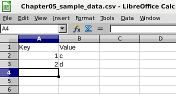
Figure 5.1 – A very simple spreadsheet example
- This will export the current worksheet to a file, as follows:
"Key","Value"
1,"c"
2,"d"
- We can then create a table to load the data into, using psql and the command:
CREATE TABLE example
(key integer
,value text);
- We can then load it into the PostgreSQL table, using the following psql command:
postgres=# COPY sample FROM sample.csv CSV HEADER
postgres=# SELECT * FROM sample;
key | value
-----+-------
1 | c
2 | d
- Alternatively, from the command line, this would be as follows:
psql -c 'COPY sample FROM sample.csv CSV HEADER'
The filename can include a full file path if the data is in a different directory. The psql COPY command transfers data from the client system where you run the command through to the database server, so the file is on the client. Higher privileges are not required, so this is the preferred method.
- If you are submitting SQL through another type of connection, then you can also use the following SQL statement of the form, noting that the leading backslash is removed:
COPY sample FROM '/mydatafiledirectory/sample.csv' CSV HEADER;
The COPY statement shown in the preceding SQL statement uses an absolute path to identify data files, which is required. This method runs on the database server and can only be executed by a super user, or a user who has been granted one of the pg_read_server_files, pg_write_server_files, or pg_execute_server_program roles. So, you need to ensure that the server process is allowed to read that file, then transfer the data yourself to the server, and finally, load the file. These privileges are not commonly granted, which is why we prefer the earlier method.
The COPY (or COPY) command does not create the table for you; that must be done beforehand. Note also that the HEADER option does nothing but ignore the first line of the input file, so the names of the columns from the .csv file don't need to match those of the Postgres table. If it hasn't occurred to you yet, this is also a problem. If you say HEADER and the file does not have a header line, then all it does is ignore the first data row. Unfortunately, there's no way for PostgreSQL to tell whether the first line of the file is truly a header or not. Be careful!
There isn't a standard tool to load data directly from the spreadsheet to the database. It's fairly simple to write a spreadsheet macro to automate the aforementioned tasks, but that's not a topic for this book.
How it works...
The COPY command executes a COPY SQL statement, so the two methods described earlier are very similar. There's more to be said about COPY, so we'll cover that in the next recipe.
Under the covers, the COPY command executes a COPY … FROM STDIN command. When using this form of command, the client program must read the file and feed the data to the server. psql does this for you, but in other contexts, you can use this mechanism to avoid the need for higher privileges or additional roles, which are needed when running COPY with an absolute filename.
There's more...
There are many data extraction and loading tools available out there, some cheap and some expensive. Remember that the hardest part of loading data from any spreadsheet is separating the data from all the other things it contains. I've not yet seen a tool that can help with that! This is why the best practice for spreadsheets is to separate data into separate worksheets.
Loading data from flat files
Loading data into your database is one of the most important tasks. You need to do this accurately and quickly. Here's how.
Getting ready
For basic loading, COPY works well for many cases, including CSV files, as shown in the last recipe.
If you want advanced functionality for loading, you may wish to try pgloader, which is commonly available in all main software distributions. At the time of writing, the current stable version is 3.6.3. There are many features, but it is stable, with very few new features in recent years.
How to do it...
To load data with pgloader, we need to understand our requirements, so let's break this down into a step-by-step process, as follows:
- Identify the data files and where they are located. Make sure that pgloader is installed in the location of the files.
- Identify the table into which you are loading, ensure that you have the permissions to load, and check the available space. Work out the file type (examples include fixed-size fields, delimited text, and CSV) and check the encoding.
- Specify the mapping between columns in the file and columns on the table being loaded. Make sure you know which columns in the file are not needed – pgloader allows you to include only the columns you want. Identify any columns in the table for which you don't have data. Do you need them to have a default value on the table, or does pgloader need to generate values for those columns through functions or constants?
- Specify any transformations that need to take place. The most common issue is date formats, although it's possible that there may be other issues.
- Write the pgloader script.
- The pgloader script will create a log file to record whether the load has succeeded or failed, and another file to store rejected rows. You need a directory with sufficient disk space if you expect them to be large. Their size is roughly proportional to the number of failing rows.
- Finally, consider what settings you need for performance options. This is definitely last, as fiddling with things earlier can lead to confusion when you're still making the load work correctly.
- You must use a script to execute pgloader. This is not a restriction; actually, it is more like a best practice, because it makes it much easier to iterate toward something that works. Loads never work the first time, except in the movies!
Let's look at a typical example from the quick-start documentation of pgloader, the csv.load file.
Define the required operations in a command and save it in a file, such as csv.load:
LOAD CSV
FROM '/tmp/file.csv' (x, y, a, b, c, d)
INTO postgresql://postgres@localhost:5432/postgres?csv (a, b, d, c)
WITH truncate,
skip header = 1,
fields optionally enclosed by '"',
fields escaped by double-quote,
fields terminated by ','
SET client_encoding to 'latin1',
work_mem to '12MB',
standard_conforming_strings to 'on'
BEFORE LOAD DO
$$ drop table if exists csv; $$,
$$ create table csv (
a bigint,
b bigint,
c char(2),
d text
);
$$;
This command allows us to load the following CSV file content. Save this in a file, such as file.csv, under the /tmp directory:
Header, with a © sign
"2.6.190.56","2.6.190.63","33996344","33996351","GB","United Kingdom"
"3.0.0.0","4.17.135.31","50331648","68257567","US","United States"
"4.17.135.32","4.17.135.63","68257568","68257599","CA","Canada"
"4.17.135.64","4.17.142.255","68257600","68259583","US","United States"
"4.17.143.0","4.17.143.15","68259584","68259599","CA","Canada"
"4.17.143.16","4.18.32.71","68259600","68296775","US","United States"
We can use the following load script:
pgloader csv.load
Here's what gets loaded in the PostgreSQL database:
postgres=# select * from csv;
a | b | c | d
----------+----------+----+----------------
33996344 | 33996351 | GB | United Kingdom
50331648 | 68257567 | US | United States
68257568 | 68257599 | CA | Canada
68257600 | 68259583 | US | United States
68259584 | 68259599 | CA | Canada
68259600 | 68296775 | US | United States
(6 rows)
How it works…
pgloader copes gracefully with errors. The COPY command loads all rows in a single transaction, so only a single error is enough to abort the load. pgloader breaks down an input file into reasonably sized chunks and loads them piece by piece. If some rows in a chunk cause errors, then pgloader will split it iteratively until it loads all the good rows and skips all the bad rows, which are then saved in a separate rejects file for later inspection. This behavior is very convenient if you have large data files with a small percentage of bad rows – for instance, you can edit the rejects, fix them, and finally, load them with another pgloader run.
Versions from the 2.x iteration of pgloader were written in Python and connected to PostgreSQL through the standard Python client interface. Version 3.x is written in Common Lisp. Yes, pgloader is less efficient than loading data files using a COPY command, but running a COPY command has many more restrictions: the file has to be in the right place on the server, has to be in the right format, and must be unlikely to throw errors on loading. pgloader has additional overhead, but it also has the ability to load data using multiple parallel threads, so it can be faster to use as well. The ability of pgloader to reformat the data via user-defined functions is often essential; a straight COPY command may not be enough.
pgloader also allows loading from fixed-width files, which COPY does not.
If you need to reload the table completely from scratch, then specify the WITH TRUNCATE clause in the pgloader script.
There are also options to specify SQL to be executed before and after loading data. For instance, you can have a script that creates the empty tables before, you can add constraints after, or both.
There's more…
After loading, if we have load errors, then there will be bloat in the PostgreSQL tables. You should think about whether you need to add a VACUUM command after the data load, though this will possibly make the load take much longer.
We need to be careful to avoid loading data twice. The only easy way of doing so is to make sure that there is at least one unique index defined on every table that you load. The load should then fail very quickly.
String handling can often be difficult because of the presence of formatting or non-printable characters. The default setting for PostgreSQL is to have a parameter named standard_conforming_strings set to off, which means that backslashes will be assumed to be escape characters. Put another way, by default, the string means a line feed, which can cause data to appear truncated. You'll need to turn standard_conforming_strings to on, or you'll need to specify an escape character in the load-parameter file.
If you are reloading data that has been unloaded from PostgreSQL, then you may want to use the pg_restore utility instead. The pg_restore utility has an option to reload data in parallel, -j number_of_threads, though this is only possible if the dump was produced using the custom pg_dump format. Refer to the recipes in Chapter 11, Backup and Recovery, for more details. This can be useful for reloading dumps, though it lacks almost all of the other pgloader features discussed here.
If you need to use rows from a read-only text file that does not have errors, then you may consider using the file_fdw contrib module. The short story is that it lets you create a virtual table that will parse the text file every time it is scanned. This is different from filling a table once and for all, either with COPY or pgloader; therefore, it covers a different use case. For example, think about an external data source that is maintained by a third party and needs to be shared across different databases.
Another option would be EDB*Loader, which also contains a wide range of load options: https://www.enterprisedb.com/docs/epas/latest/epas_compat_tools_guide/02_edb_loader/.
Making bulk data changes using server-side procedures with transactions
In some cases, you'll need to make bulk changes to your data. In many cases, you need to scroll through the data making changes according to a complex set of rules. You have a few choices in that case:
- Write a single SQL statement that can do everything.
- Open a cursor and read the rows out, and then make changes with a client-side program.
- Write a procedure that uses a cursor to read the rows and make changes using server-side SQL.
Writing a single SQL statement that does everything is sometimes possible, but if you need to do more than just use UPDATE, then it becomes difficult very quickly. The main difficulty is that the SQL statement isn't restartable, so if you need to interrupt it, you will lose all of your work.
Reading all the rows back to a client-side program can be very slow – if you need to write this kind of program, it is better to do it all on the database server.
Getting ready
Create an example table and fill it with nearly 1,000 rows of test data:
CREATE TABLE employee (
empid BIGINT NOT NULL PRIMARY KEY
,job_code TEXT NOT NULL
,salary NUMERIC NOT NULL
);
INSERT INTO employee VALUES (1, 'A1', 50000.00);
INSERT INTO employee VALUES (2, 'B1', 40000.00);
INSERT INTO employee SELECT generate_series(10,1000), 'A2', 10000.00);
How to do it…
We're going to write a procedure in PL/pgSQL. A procedure is similar to a function, except that it doesn't return any value or object. We use a procedure because it allows you to run multiple server-side transactions. By using procedures in this way, we are able to break the problem down into a set of smaller transactions that cause less of a problem with database bloat and long-running transactions.
As an example, let's consider a case where we need to update all employees with the A2 job grade, giving each person a 2% pay rise:
CREATE PROCEDURE annual_pay_rise (percent numeric)
LANGUAGE plpgsql AS $$
DECLARE
c CURSOR FOR
SELECT * FROM employee
WHERE job_code = 'A2';
BEGIN
FOR r IN c LOOP
UPDATE employee
SET salary = salary * (1 + (percent/100.0))
WHERE empid = r.empid;
IF mod (r.empid, 100) = 0 THEN
COMMIT;
END IF;
END LOOP;
END;
$$;
Execute the preceding procedure like this:
CALL annual_pay_rise(2);
We want to issue regular commits as we go. The preceding procedure is coded so that it issues commits roughly every 100 rows. There's nothing magical about that number; we just want to break it down into smaller pieces, whether it is the number of rows scanned or rows updated.
There's more…
You can use both COMMIT and ROLLBACK in a procedure. Each new transaction will see the changes from prior transactions and any other concurrent commits that have occurred.
What happens if your procedure is interrupted? Since we are using multiple transactions to complete the task, we won't expect the whole task to be atomic. If the execution is interrupted, we need to rerun the parts that didn't execute successfully. What happens if we accidentally rerun parts that have already been executed? We will give some people a double pay rise, but not everyone.
To cope, let's invent a simple job restart mechanism. This uses a persistent table to track changes as they are made, accessed by a simple API:
CREATE TABLE job_status
(id bigserial not null primary key,status text not null,restartdata bigint);
CREATE OR REPLACE FUNCTION job_start_new ()
RETURNS bigint
LANGUAGE plpgsql
AS $$
DECLARE
p_id BIGINT;
BEGIN
INSERT INTO job_status (status, restartdata)
VALUES ('START', 0)
RETURNING id INTO p_id;
RETURN p_id;
END; $$;
CREATE OR REPLACE FUNCTION job_get_status (jobid bigint)
RETURNS bigint
LANGUAGE plpgsql
AS $$
DECLARE
rdata BIGINT;
BEGIN
SELECT restartdata INTO rdata
FROM job_status
WHERE status != 'COMPLETE' AND id = jobid;
IF NOT FOUND THEN
RAISE EXCEPTION 'job id does not exist';
END IF;
RETURN rdata;
END; $$;
CREATE OR REPLACE PROCEDURE
job_update (jobid bigint, rdata bigint)
LANGUAGE plpgsql
AS $$
BEGIN
UPDATE job_status
SET status = 'IN PROGRESS'
,restartdata = rdata
WHERE id = jobid;
END; $$;
CREATE OR REPLACE PROCEDURE job_complete (jobid bigint)
LANGUAGE plpgsql
AS $$
BEGIN
UPDATE job_status SET status = 'COMPLETE'
WHERE id = jobid;
END; $$;
First of all, we start a new job:
SELECT job_start_new();
Then, we execute our procedure, passing the job number to it. Let's say this returns 8474:
CALL annual_pay_rise(8474);
If the procedure is interrupted, we will restart from the correct place, without needing to specify any changes:
CALL annual_pay_rise(8474);
The existing procedure needs to be modified to use the new restart API, as shown in the following code block. Note, also, that the cursor has to be modified to use an ORDER BY clause to make the procedure sensibly repeatable:
CREATE OR REPLACE PROCEDURE annual_pay_rise (job bigint)
LANGUAGE plpgsql AS $$
DECLARE
job_empid bigint;
c NO SCROLL CURSOR FOR
SELECT * FROM employee
WHERE job_code='A2'
AND empid > job_empid
ORDER BY empid;
BEGIN
SELECT job_get_status(job) INTO job_empid;
FOR r IN c LOOP
UPDATE employee
SET salary = salary * 1.02
WHERE empid = r.empid;
IF mod (r.empid, 100) = 0 THEN
CALL job_update(job, r.empid);
COMMIT;
END IF;
END LOOP;
CALL job_complete(job);
END; $$;
For extra practice, follow the execution using the debugger in pgAdmin or OmniDB.
The CALL statement can also be used to call functions that return void, but other than that, functions and procedures are separate concepts. Procedures also allow you to execute transactions in PL/Python and PL/Perl.