5

Understanding AutoML Algorithms

All ML algorithms have a foundation in computational statistics. Computational statistics is the combination of statistics and computer science where computers are used to compute complex mathematics. This computation is the ML algorithm and the results that we get from it are the predictions. As engineers and scientists working in the field of ML, we are often expected to know the basic logic of ML algorithms. There are plenty of ML algorithms in the AI domain. All of them aim to solve different types of prediction problems. All of them also have their own set of pros and cons. Thus, it became the job of engineers and scientists to find the best ML algorithms that can solve a given prediction problem within the required constraints. This job, however, was eased with the invention of AutoML.

Despite AutoML taking over this huge responsibility of finding the best ML algorithm, it is still our job as engineers and scientists to verify and justify the selection of these algorithms. And to do that, a basic understanding of the ML algorithms is a must.

In this chapter, we shall explore and understand the various ML algorithms that H2O AutoML uses to train models. As mentioned previously, all ML algorithms have a heavy foundation in statistics. Statistics itself is a huge branch of mathematics and is too large to cover in a single chapter. Hence, for the sake of having a basic understanding of how ML algorithms work, we shall explore their inner workings conceptually with basic statistics rather than diving deep into the math.

Tip

If you are interested in gaining more knowledge in the field of statistics, then the following link should be a good place to start: https://online.stanford.edu/courses/xfds110-introduction-statistics.

First, we shall understand what the different types of ML algorithms are and then learn about the workings of these algorithms. We will do this by breaking them down into individual concepts, understanding them, and then building the algorithm back up to understand the big picture.

In this chapter, we are going to cover the following topics:

• Understanding the different types of ML algorithms
• Understanding the Generalized Linear Model algorithm
• Understanding the Distributed Random Forest algorithm
• Understanding the Gradient Boosting Machine algorithm
• Understanding what is Deep Learning

So, let’s begin our journey by understanding the different types of ML algorithms.

Understanding the different types of ML algorithms

ML algorithms are designed to solve a specific prediction problem. These prediction problems can be anything that can provide value if predicted accurately. The differentiating factor between various prediction problems is what value is to be predicted. Is it a simple yes or no value, a range of numbers, or a specific value from a list of potential values, probabilities, or semantics of a text? The field of ML is vast enough to cover the majority, if not all, of such problems in a wide variety of ways.

So, let’s start with understanding the different categories of prediction problems. They are as follows:

• Regression: Regression analysis is a statistical process that aims to find the relationship between independent variables, also called features, and dependent variables, also called label or response variables, and use that relationship to predict future values.

Regression problems are problems that aim to predict certain continuous numerical values – for example, predicting the price of a car given the car’s brand name, engine size, economy, and electronic features. In such a scenario, the car’s brand name, engine size, economy, and electronic features are the independent variables as their presence is independent of other values, while the car price is the dependent variable whose value is dependent on the other features. Also, the price of the car is a continuous value as it can numerically range anywhere from 0 to 100 million in dollars or any other currency.

• Classification: Classification is a statistical process that aims to categorize the label values depending on their relationship to the features into certain classes or categories.

Classification problems are problems that aim to predict a certain set of values – for example, predicting if a person is likely to face heart disease, depending on their cholesterol level, weight, exercise levels, heart rate, and family history. Another example would be predicting the rating of a restaurant on Google reviews that ranges from 1-5 stars, depending on the location, food, ambience, and price.

As you can see from these examples, classification problems can be either a yes or no, true or false, or 1 or 0 type of classification, or a specific set of classification values, such as those in the Google Review example, where the values can either be 1, 2, 3, 4, or 5. Thus, classification problems can be further divided, as follows:

• Binary Classification: In this type of classification problem, the predicted values are binary, meaning they have only two values – that is, yes or no, true or false, 1 or 0.
• Multiclass/Polynomial Classification: In this type of classification problem, the predicted values are non-binary, also called polynomial, in nature, meaning they have more than two sets of values. For example, classification by age, which involves whole numbers from 1 to 100, or classification by primary colors, which can be red, yellow, or blue.

• Clustering: Clustering is a statistical process that aims to group or divide certain data points in such a way that data points in a single group have similar characteristics that are different from data points in other groups.

Clustering problems are problems that aim to understand similarities within a set of values.

For example, given a set of people who play video games with certain details, such as the hardware they use, the different games they play, and time spent playing those video games, you can categorize people by their favorite game genre. Clustering can be further divided as follows:

• Hard Clustering: In this type of clustering, all data points either belong to one or another cluster; they are mutually exclusive.
• Soft Clustering: In this type of clustering, rather than assigning a data point to a cluster, the probability that a data point might belong to a certain cluster is calculated. This opens the likelihood that a data point might belong to multiple clusters at the same time.

• Association: Association is a statistical process that aims to find the probability that if event A happened, what is the likelihood that event B will happen too? Association problems are based on association rules, which are if-then statements that show the probability of a relationship between different data points.

The most common example of the association problem is Market Basket Analysis. Market Basket Analysis is a prediction problem where, given a user buys a certain product A from the market, what is the probability of the user buying product B, which is related to product A?

• Optimization/Control: Control Theory, Optimal Control Theory, or Optimization Problems is a branch of mathematics that deals with finding a certain combination of values that collectively optimize a dynamic system. Machine Learning Control (MLC) is a subfield in ML that aims to solve the Optimization Problem using ML. A good example of MLC is the implementation of ML to optimize traffic on roads using automated cars.

Now that we understand the different types of prediction problems, let’s dive into understanding the different types of ML algorithms. The different types of ML algorithms are categorized as follows:

• Supervised Learning: Supervised learning is the ML task of mapping the relationship between the independent variables and dependent variables based on previously existing values that are labeled. Labeled data is data that contains information about which of its features are dependent and which features are independent. In supervised learning, we know which feature we want to predict and tag that feature as a label. The ML algorithm will use this information to map the relationships. Using this mapping, we predict the output for new input values. Another way of understanding this problem is that the previously existing values supervise the ML algorithm's learning task.

Supervised learning algorithms are often used to solve regression and classification problems.

Some examples of supervised learning algorithms are decision trees, linear regression, and neural networks.

• Unsupervised learning: As mentioned previously, supervised learning is the ML task of finding patterns and behaviors from data that is not tagged. In this case, we don’t know which feature we want to predict, or the feature we want to predict may not even be a part of the dataset. Unsupervised learning helps us predict potential repeating patterns and categorize the set of data using those patterns. Another way of understanding this problem is that there are no labeled values to supervise the ML algorithm learning task; the algorithm learns the patterns and behaviors on its own.

Unsupervised learning algorithms are often used to solve clustering and association problems.

Some examples of unsupervised learning algorithms are K-means clustering and association rule learning.

• Semi-supervised learning: Semi-supervised learning falls between supervised learning and unsupervised learning. It is the ML task of performing learning on a dataset that is partially labeled. It is used in scenarios where you have a small dataset that is labeled along with a large unlabeled dataset. In real-world scenarios, labeling large amounts of data is an expensive task as it requires a lot of experimentation and contextual information that is manually interpreted, while unlabeled data is relatively cheap to acquire. Semi-supervised learning often proves efficient in this case as it is good at assuming expected label values from unlabeled datasets while working as efficiently as any supervised learning algorithm.

Unsupervised learning algorithms are often used to solve clustering and classification problems.

Some examples of semi-supervised learning algorithms are generative models and Laplacian regularization.

• Reinforcement learning: Reinforcement learning is an ML task that aims to identify the next correct logical action to take in a given environment to maximize the cumulative reward. In this type of learning, the accuracy of the prediction is calculated after the prediction is made using positive and/or negative reinforcement, which is again fed to the algorithm. This continuous learning of the environment eventually helps the algorithm find the best sequence of steps to take to maximize the reward, thus making the most accurate decision.

Reinforcement learning is often used to solve a mix of regression, classification, and optimization problems.

Some examples of reinforcement learning algorithms are Monte Carlo Methods, Q-Learning, and Deep Q Network.

The AutoML technology, despite being mature enough to be used commercially, is still in its infancy compared to the vast developments in the field of ML. AutoML may be able to train the best predictive models in the shortest time using little to no human intervention, but its potential is currently limited to only supervised learning. The following diagram summarizes the various types of ML algorithms categorized under the different ML tasks:

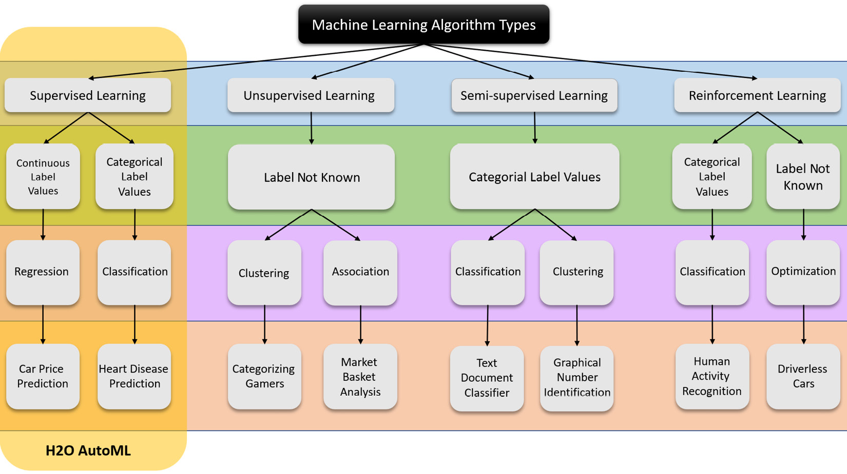
Figure 5.1 – Types of ML problems and algorithms

Similarly, H2O’s AutoML also focuses on supervised learning and as such, you are often expected to have labeled data that you can feed to it.

ML algorithms that perform unsupervised learning are often quite sophisticated compared to supervised learning algorithms as there is no ground truth to measure the performance of the model. This goes against the very nature of AutoML, which is very reliant on model performance measurements to automate training and hyperparameter tuning.

So, accordingly, H2O AutoML falls in the domain of supervised ML algorithms, where it trains several supervised ML algorithms to solve regression and classification problems and ranks them based on their performance. In this chapter, we shall focus on these ML algorithms and understand their functionality so that we are well equipped to understand, select, and justify the different models that H2O AutoML trains for a given prediction problem.

With this understanding, let’s start with the first ML algorithm: Generalized Linear Model.

Understanding the Generalized Linear Model algorithm

Generalized Linear Model (GLM), as its name suggests, is a flexible way of generalizing linear models. It was formulated by John Nelder and Robert Wedderburn as a way of combining various regression models into a single analysis with considerations given to different probability distributions. You can find their detailed paper (Nelder, J.A. and Wedderburn, R.W., 1972. Generalized linear models. Journal of the Royal Statistical Society: Series A (General), 135(3), pp.370-384.) at https://rss.onlinelibrary.wiley.com/doi/abs/10.2307/2344614.

Now, you may be wondering what linear models are. Why do we need to generalize them? What benefit does it provide? These are relevant questions indeed and they are pretty easy to understand without diving too deep into the mathematics. Once we break down the logic, you will notice that the concept of GLM is pretty easy to understand.

So, let’s start by understanding the basics of linear regression.

Introduction to linear regression

Linear regression is probably one of the oldest statistical models, dating back to 200 years ago. It is an approach that maps the relationship between the dependent and independent variables linearly on a graph. What that means is that the relationship between the two variables can be completely explained by a straight line.

Consider the following example:

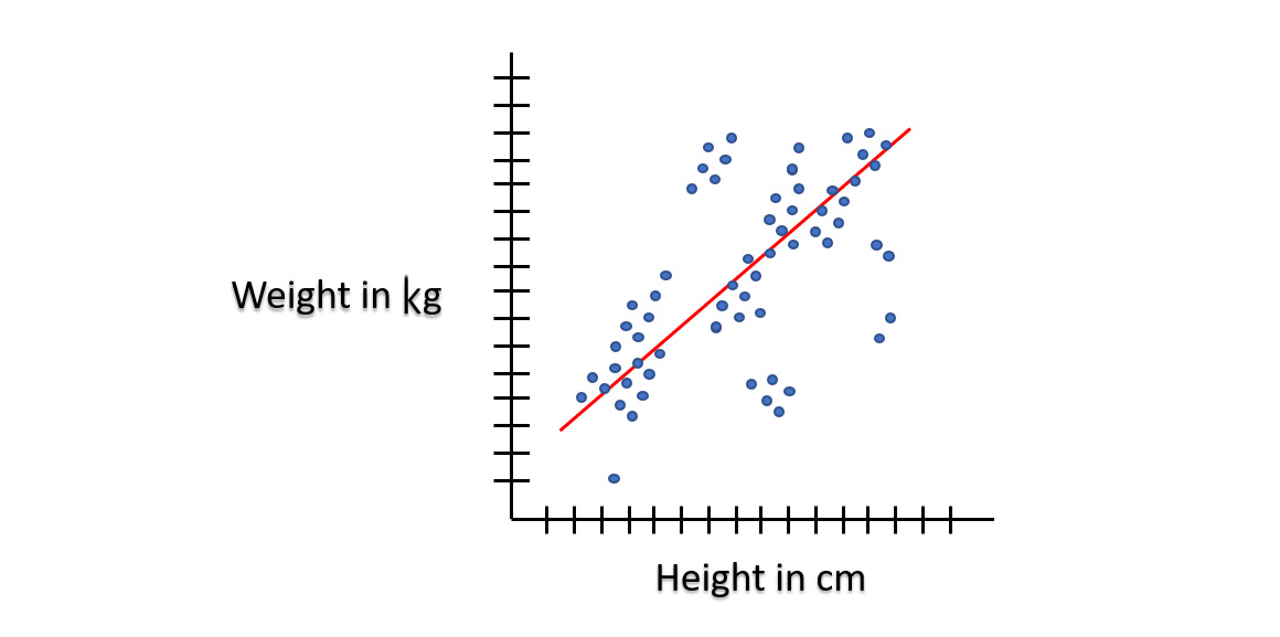
Figure 5.2 – Linear regression

This example demonstrates the relationship between two variables. The height of a person, H, is an independent variable, while the weight of a person, W, is a dependent variable. The relationship between these two variables can easily be explained by a straight red line. The taller a person is, the more likely he or she will weigh more. Easy enough to understand.

Statistically, the general equation for any straight line, also called the linear equation, is as follows:

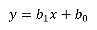
Here, we have the following:

• y is a point on the Y-axis and indicates the dependent variable.
• x is a point on the X-axis and indicates the independent variable.
• b1 is the slope of the line, also called the gradient, and indicates how steep the line is. The bigger the gradient, the steeper the line.
• b0 is a constant that indicates the point at which the line crosses the Y-axis.

During linear regression, the machine will map all the data points of the two variables on the graph and randomly place the line on the graph. Then, it will calculate the values of y by inserting the value of x from the data points in the graph into the linear equation and comparing the result with the respective y values from the data points. After that, it will calculate the magnitude of the error between the y value it calculated and the actual y value. This difference in values is what we call a residual.

The following diagram should help you understand what residuals are:

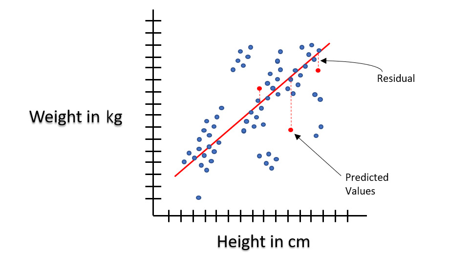
Figure 5.3 – Residuals in linear regression

The machine will do this for all the data points and make a note of all the errors. It will then try to tweak the line by changing the values of b1 and b0, meaning changing the angle and position of the line on the graph, and repeating the process. It will do this until it minimizes the error.

The values of b1 and b0 that generate the least amount of error are the most accurate linear relationship between the two variables. The equation with these values for b1 and b0 is the linear model.

Now, say you want to predict how much a person would weigh if they were 180 cm tall. Then, you use this same linear model equation with the b1 and b0 values, set x to 180, and calculate y, which will be the expected weight.

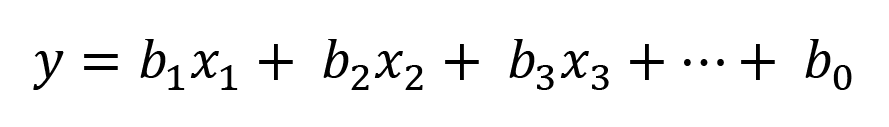
Congratulations, you just performed ML in your mind without any computers and made predictions too! Actual ML works the same way, albeit with added complexities from complex algorithms. Linear regression doesn’t need to be restricted to just two variables – it can also work on multiple variables where there’s more than one independent variable. Such linear regression is called multiple or curvilinear regression. The equation of such a linear regression expands as follows:

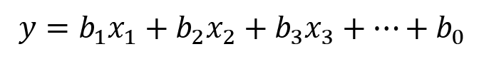
In this equation, the additional variables – x1, x2, x3, and so on – are added with their own coefficients – b1, b2, and b3, respectively.

Feel free to explore these algorithms and the mathematics behind them if you are interested in the inner workings of linear regression.

Understanding the assumptions of linear regression

Linear regression, when training a model on a given dataset, works on certain assumptions about the data. One of these assumptions is the normality of errors.

Before we understand what the normality of errors is, let’s quickly understand the concept of the probability density function. This is a mathematical expression that defines the probability distribution of discrete values – in other words, it is a mathematical expression that shows the probability of a sample value occurring from a given sample space. To understand this, refer to the following diagram:

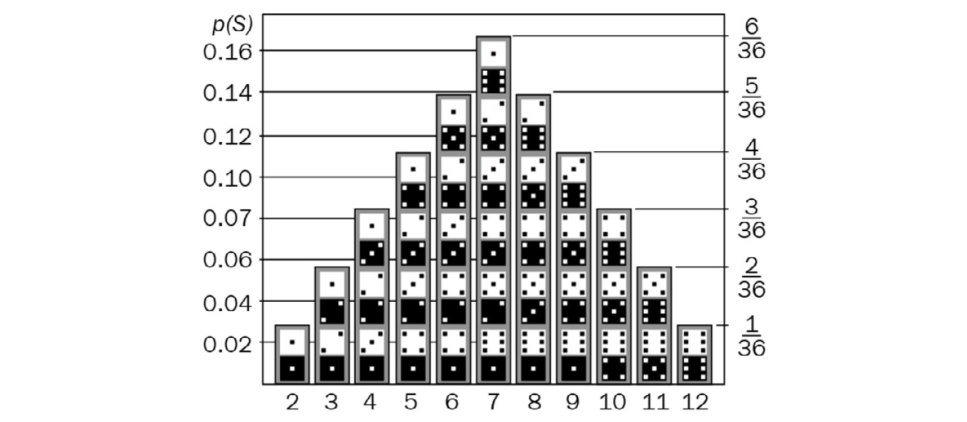
Figure 5.4 – Probability distribution of values for two dice

The preceding diagram shows the distribution of probabilities of all the values that can occur when a pair of six-sided dice are thrown fairly and independently. There are different kinds of distributions. Some examples of commonly occurring distributions are as follows:

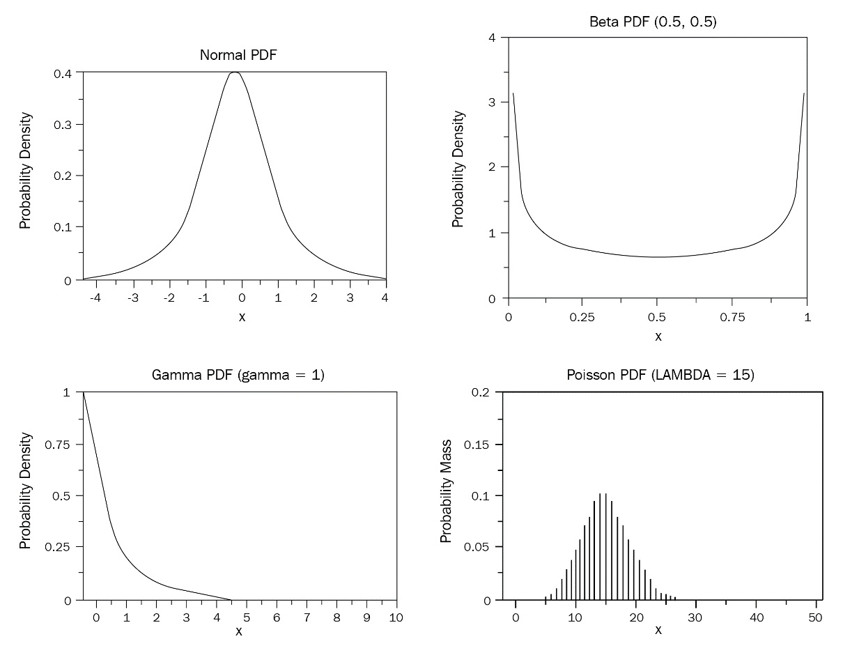
Figure 5.5 – Different types of distribution

The normality of errors states that the residuals of the data must be normally distributed. A normal distribution, also called Gaussian distribution, is a probability density function that is symmetrical about the mean, where the values closest to the mean occur frequently, while those far from the mean rarely occur. The following diagram shows a normal distribution:

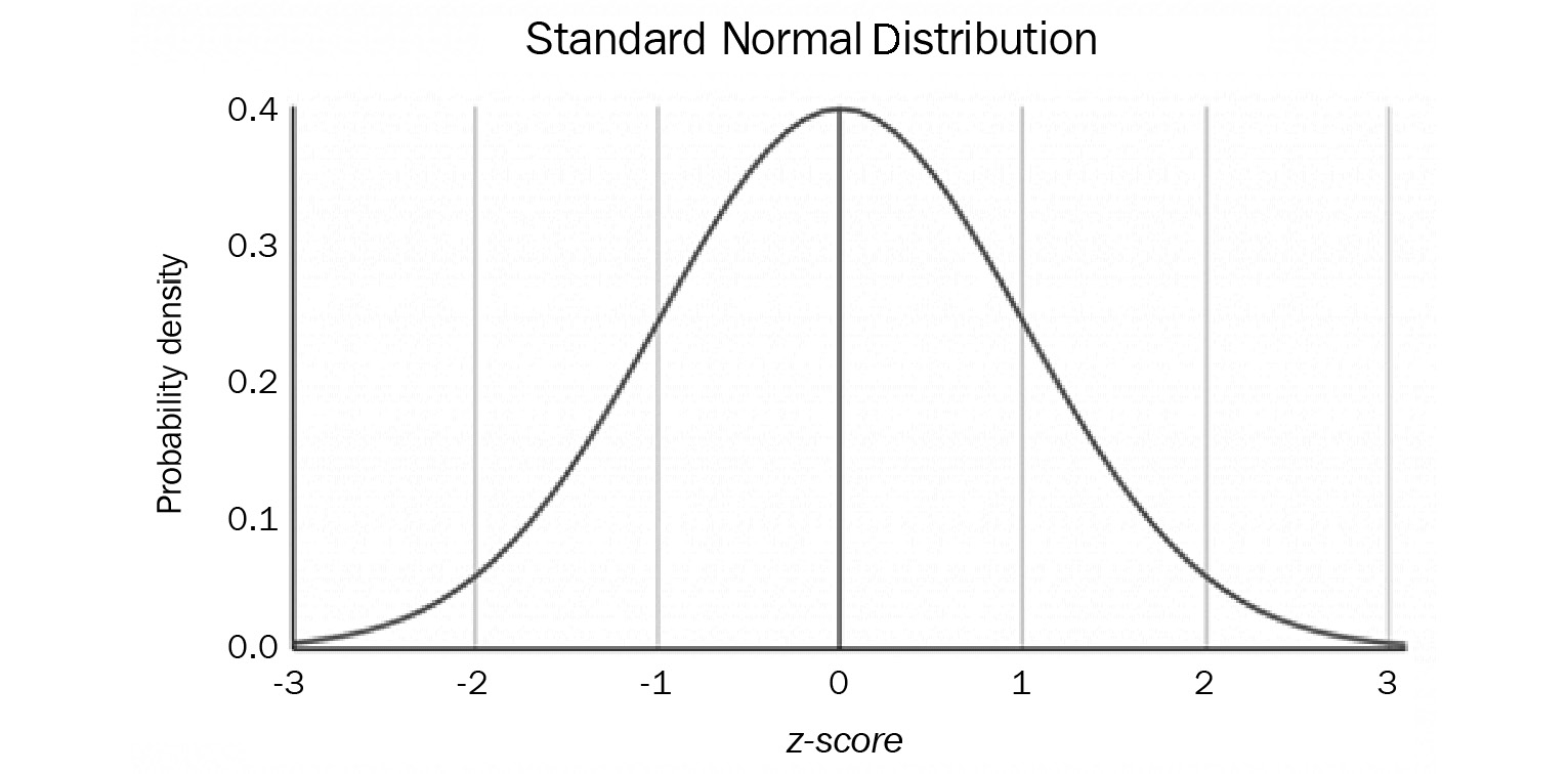
Figure 5.6 – Normal distribution

Linear regression expects the residuals that get calculated to fall within a normal distribution. In our previous example of the expected weight for a height, there is bound to be some error between the predicted weight and the actual weight of a person with a certain height. However, the residuals or errors from the prediction will most likely fall within a normal distribution as there cannot be too many occurrences of people with an extreme difference between the expected weight and the predicted weight.

Consider a scenario of people claiming health insurance payouts. The following diagram shows a sample of the linear regression graph for that dataset:

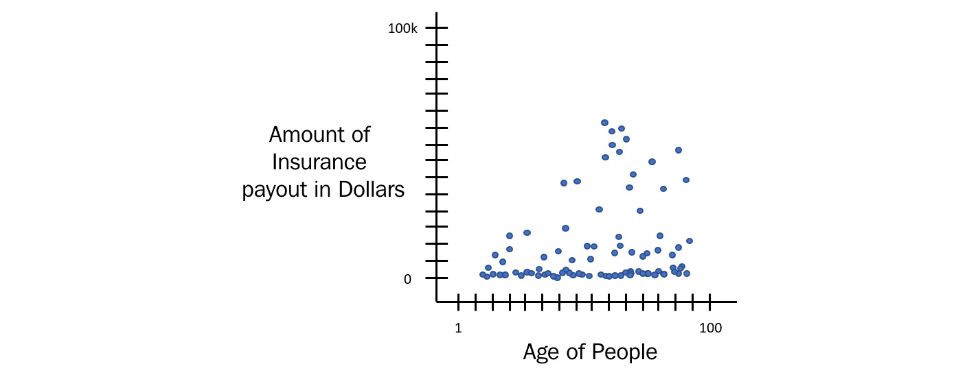
Figure 5.7 – Health insurance payout

In the preceding diagram, you can see that the majority of people from various age groups did not claim health insurance. Some of them did and the cost of claims varied a lot. Some had minor issues costing little, while some had serious injuries and had to go through expensive surgeries.

If you plot a linear regression line through this dataset, it will look as follows:

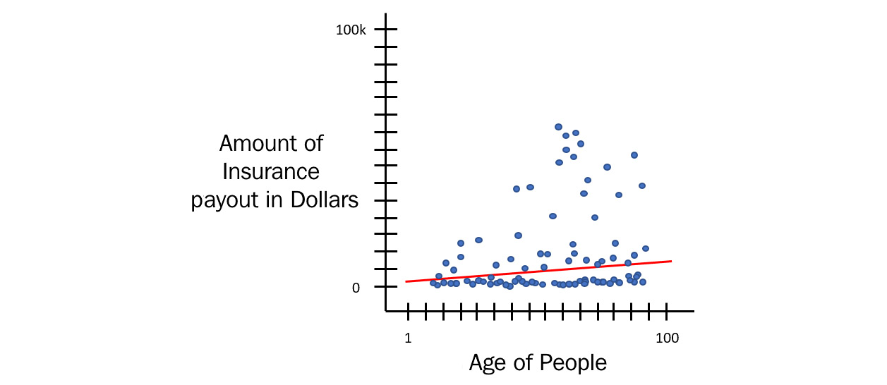
Figure 5.8 – Linear regression on health insurance payouts

But now, if you calculate the residual errors from the expected and predicted value for all the data points, then the probability distribution of these residuals will not fall into a normal distribution. It will look as follows:

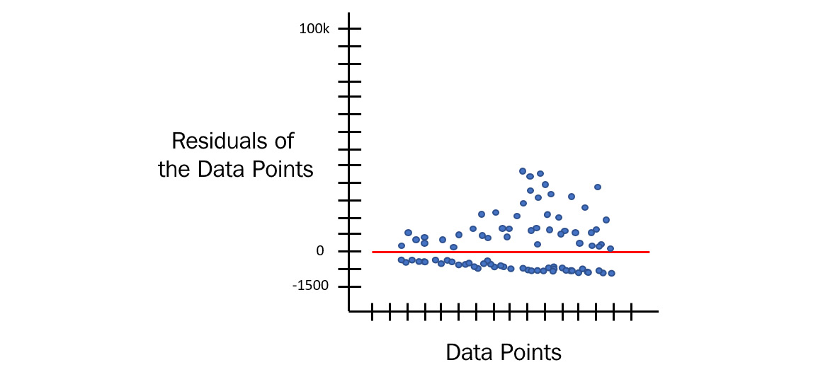
Figure 5.9 – Residual distribution of health insurance payouts

This is an inaccurate model as the expected value and the predicted values are not even close enough to round off or correct. So, what do you do for such a scenario, where the normality of errors assumption fails for the dataset? What if the distribution of the residuals is, say, Poisson instead of normal? How will the machine correct that?

Well, the answer to this is that the distribution of residuals depends on the distribution of the dataset itself. If the values of the dependent variables are normally distributed, then the distribution of the residuals will also be normal. So, once we have identified which probability density function fits the dataset, we can use that function to train our linear model.

Depending on this function, there are specialized linear regression methods for every probability density function. If your distribution is Poisson, then you can use Poisson regression. If your data distribution is negative binomial, then you can use negative binomial regression.

Working with a Generalized Linear Model

Now that we have covered the basics, let’s focus on understanding what GLM is. GLM is a way of pointing to all the regression methods that are specific to the type of probability distribution of the data. Technically, all the regression models are GLM, including our ordinary simple linear model. GLM just encapsulates them together and trains the appropriate regression model based on the probability distribution function.

The way GLM works is by using something called a link function in conjunction with a systematic component and the random variable.

These are three components of GLM:

• Systematic component: Going back to the multi-variate linear equation, we have the following:

Here, b1x1+ b2x2 + b3x3 + ……. + b0 is the systematic component. This is the function that links our data, also called predictors, with our predictions.

• Random Component: This component refers to the probability distribution of the response variable. This will be whether the response variable is normally distributed or binomially distributed or any other form of distribution.
• Link function: A link function is a function that maps the non-linear relationship of data to a linear one. In other words, it bends the line of linear regression to represent the relationship of non-linear data more accurately. It is a link between the random and the systematic components. We can explain the equation with a link function mathematically as Y = fn( b1x1+ b2x2 + b3x3 + ……. + b0 ), where fn is the link function that changes as per the distribution of the response variable.

The link function is different for different distributions. The following table shows the different link functions for different distributions:

Distribution Type	Link Function	Name of Algorithm
Normal		Linear model
Binomial		Logistic regression
Poisson		Poisson regression
Gamma		Gamma regression

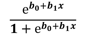
Figure 5.10 – Link functions for different distribution types

When training GLM models, you have the option of selecting the value for the family hyperparameter. The family option specifies the probability distribution of your response column and the GLM training algorithm uses the appropriate link function during training.

The values for the family hyperparameter are as follows:

• gaussian: You should select this option if the response is a real integer number.
• binomial: You should select this option if the response is categorical with two classes or binaries that could be either enums or integers.
• fractionalbinomial: You should select this option if the response is numeric between 0 and 1.
• ordinal: You should select this option if the response is a categorical response with three or more classes.
• quasibinomial: You should select this option if the response is numeric.
• multinomial: You should select this option if the response is a categorical response with three or more classes that are of enum types.
• poisson: You should select this option if the response is numeric and contains non-negative integers.
• gamma: You should select this option if the response is numeric and continuous and contains positive real integers.
• tweedie: You should select this option if the response is numeric and contains continuous real values and non-negative values.
• negativebinomial: You should select this option if the response is numeric and contains a non-negative integer.
• AUTO: This determines the family automatically for the user.

As you may have guessed, H2O’s AutoML selects AUTO as the family type when training GLM models. The AutoML process handles this case of selecting the correct distribution family by understanding the distribution of the response variable in the dataset and applying the correct link function to train the GLM model.

Congratulations, we have just looked into how the GLM algorithm works! GLM is a very powerful and flexible algorithm and H2O AutoML expertly configures its training so that it trains the most accurate and high-performance GLM model.

Now, let’s move on to the next ML algorithm that H2O trains: Distributed Random Forest (DRF).

Understanding the Distributed Random Forest algorithm

DRF, simply called Random Forest, is a very powerful supervised learning technique often used for classification and regression. The foundation of the DRF learning technique is based on decision trees, where a large number of decision trees are randomly created and used for predictions and their results are combined to get the final output. This randomness is used to minimize the bias and variance of all the individual decision trees. All the decision trees are collectively combined and called a forest, hence the name Random Forest.

To get a deeper conceptual understanding of DRF, we need to understand the basic building block of DRF – that is, a decision tree.

Introduction to decision trees

In very simple terms, a decision tree is just a set of IF conditions that either return a yes or a no answer based on data passed to it. The following diagram shows a simple example of a decision tree:

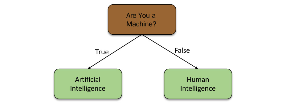
Figure 5.11 – Simple decision tree

The preceding diagram shows a basic decision tree. A decision tree consists of the following components:

• Nodes: Nodes are basically IF conditions that split the decision tree based on whether the condition was met or not.
• Root Node: The node on the top of the decision tree is called the root node.
• Leaf Node: The nodes of the decision tree that do not branch out further are called leaf nodes, or simply leaves. The condition, in this case, is if the value of the data that’s passed to it is numeric, then the answer is the data is a number; if the data that’s passed to it is not numeric, then the answer will be the data is non-numeric. This is simple enough to understand.

As seen in Figure 5.11, the decision tree is based on a simple true or false question. Decision trees can also be based on mathematical conditions on numeric data. The following example shows a decision tree on numeric conditions:

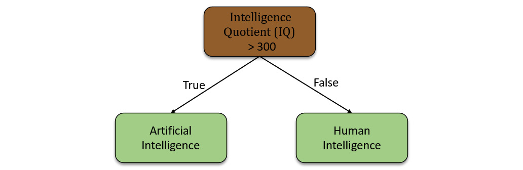
Figure 5.12 – Numerical decision tree

In this example, the root node computes whether the IQ number is greater than 300 and decides if it is artificial intelligence or human intelligence.

Decision trees can be combined as well. They can form a complex set of decision-making conditions that rely on the results of previous decisions. Refer to the following example for a complex decision tree:

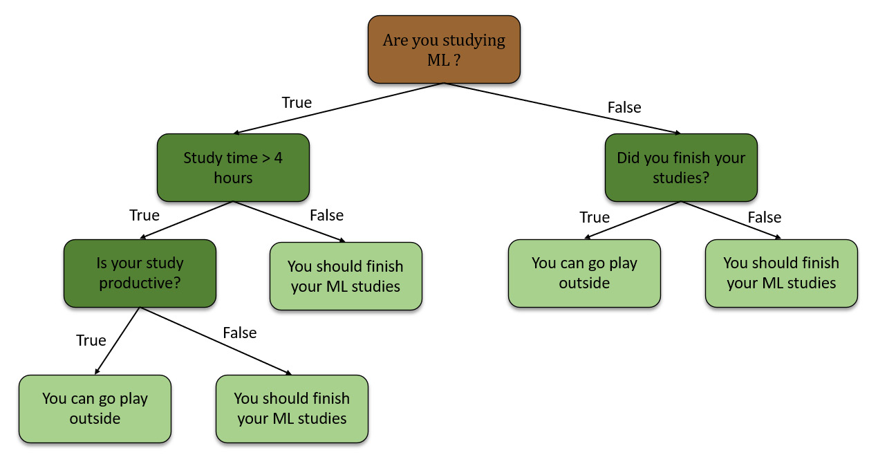
Figure 5.13 – Complex decision tree

In the preceding example, we are trying to calculate if you can go play outside or finish your ML studies. This decision tree combines numeric data as well as the classification of data. When making predictions, the decision tree will start at the top and work its way down, making decisions on whether the data satisfies the conditions or not. The leaf nodes are the final potential results of the decision tree.

With this knowledge in mind, let’s create a decision tree on a sample dataset. Refer to the following table for the sample dataset:

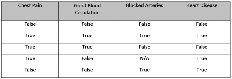
Figure 5.14 – Sample dataset for creating a decision tree

The content of the aforementioned dataset is as follows:

• Chest Pain: This column indicates if a patient suffers from chest pain.
• Good Blood Circulation: This column indicates if a patient has good blood circulation.
• Blocked Arteries: This column indicates if a patient has any blocked arteries.
• Heart Disease: This column indicates if the patient suffers from heart disease.

For this scenario, we want to create a decision tree that uses Chest Pain, Good Blood Circulation, and Blocked Arteries features to predict whether a patient has heart disease. Now, when forming a decision tree, the first thing that we need to do is find the root node. So, what feature should we place at the top of the decision tree?

We start by looking at how the Chest Pain feature alone fairs when predicting heart disease. We shall go through all the values in the dataset and map them to this decision tree while comparing the values in the Chest Pain column with those of heart disease. We shall keep track of these relationships in the decision tree. The decision tree for Chest Pain as the root node will be as follows:

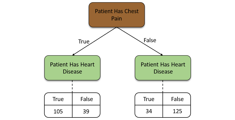
Figure 5.15 – Decision tree for the Chest Pain feature

Now, we do this for all the other features in the dataset. We create a decision tree for Good Blood Circulation and see how it fairs alone when making predictions for Heart Disease and keep a track of the comparison, repeating the same process for the Blocked Arteries status as well. If there are any missing values in the dataset, then we skip them. Ideally, you should not work with datasets that have missing values. We can use the techniques we learned about in Chapter 3, Understanding Data Processing, where we impute and handle missing dataset values.

Refer to the following diagram, which shows the two decision trees that were created – one for Patient Has Blocked Arteries and another for Patient Has Good Blood Circulation:

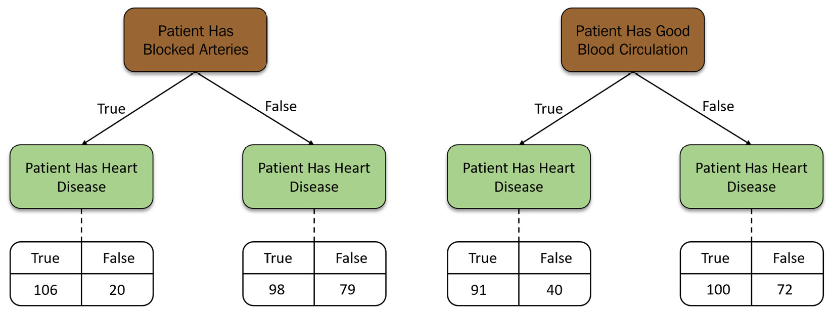
Figure 5.16 – Decision tree for the Blocked Arteries and Good Blood Circulation features

Now that we have created a decision tree for all the features in the dataset, we can compare their results to find the pure feature. In the context of decision trees, a feature is said to be 100% impure when a node is split evenly, 50/50, and 100% pure when all of its data belongs to a single class. In our scenario, we don’t have any feature that is 100% pure. All of our features are impure to some degree. So, we need to find some way of finding the feature that is the purest. For that, we need a metric that can measure the purity of a decision tree.

There are plenty of ways by which data scientists and engineers measure purity. The most common metric to measure impurity in decision trees is Gini Impurity. Gini Impurity is the measure of the likelihood that a new random instance of data will be incorrectly classified during classification.

Gini Impurity is calculated as follows:

Here, p1, p2 , p3 , p4 … are the probabilities of the various classifications for Heart Disease. In our scenario, we only have two classifications – either a yes or a no. Thus, for our scenario, the measure of impurity is as follows:

So, let’s calculate the Gini Impurity of all the decision trees we just created so that we can find the feature that is the purest. Gini Impurity for a decision tree with multiple leaf nodes is calculated by calculating the Gini Impurity of individual leaf nodes and then calculating the weighted average of all the impurity values to get the Gini Impurity of the decision tree as a whole. So, let’s start by calculating the Gini Impurity of the left leaf node of the Chest Pain decision tree and repeat this for the right leaf node:

The reason why we calculate the weighted average of the Gini Impurities is because the representation of the data is not equally divided between the two branches of the decision tree. The weighted average helps us offset this unequal distribution of the data values. Thus, we can calculate the Gini Impurity of the whole Chest Pain decision tree as follows:

Gini Impurity (Chest Pain) = weighted average of the Gini Impurities of the leaf nodes

Gini Impurity (Chest Pain) =

(Total number of data inputs in the left leaf node / total number of rows) x Gini Impurity of the left leaf node

+

(Total number of data inputs in the right leaf node / total number of rows) x Gini Impurity of the right leaf node

= (144 / (144 + 159)) x 0.395 + (159 / (144 + 159)) x 0.364

= 0.364

The Gini Impurity of the Chest Pain decision tree is 0.364.

We repeat this process for all the other feature decision trees as well. We should get the following results:

• The Gini Impurity of the Chest Pain decision tree is 0.364
• The Gini Impurity of the Good Blood Circulation tree is 0.360
• The Gini Impurity of the Blocked Arteries tree is 0.381

Comparing these values, we can infer that the Gini Impurity of the Good Blood Circulation feature has the lowest Gini Impurity, making it the purest feature in the dataset. So, we will use it as the root of our decision tree.

Referring to Figures 5.12 and 5.13, when we divided the patients by using the Good Blood Circulation feature, we were left with an impure distribution of the results on the left and right leaf nodes. So, each leaf node had a mix of results that showed with and without Heart Disease. Now, we need to figure out a way to separate the mix of results from the Good Blood Circulation feature using the remaining features – Chest Pain and Blocked Arteries.

So, just as how we did previously, we shall use these mixed results and separate them using the other features and calculate the Gini Impurity value of those features. We shall choose the feature that is the purest and replace it at the given node for further classification.

We shall repeat this process for the right branch as well. So, to simplify the selection of the decision tree nodes, we must do the following:

• Calculate the Gini Impurity score of all the remaining features for that node using the mixed results.
• Choose the one with the lowest impurity and replace it with the node.
• Repeat the same process further down the decision tree with the remaining features.
• Continue replacing the nodes, so long as the classification lowers the Gini Impurity; otherwise, leave it as a leaf node.

So, your final decision tree will be as follows:

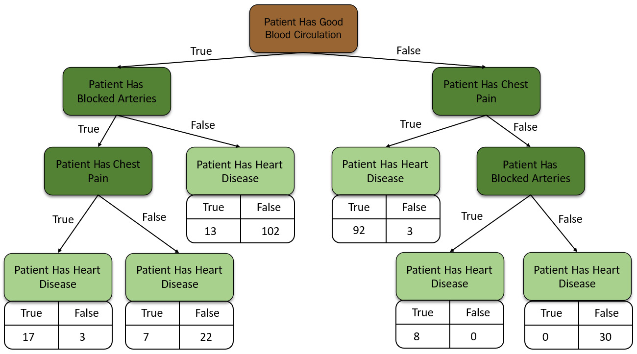
Figure 5.17 – The final decision tree

This decision tree is good for classification with true or false values. What if you had numerical data instead?

Creating decision trees with numerical data is very easy and has almost the same steps as we do for true/false data. Consider Weight as a new feature; the data for the Weight column is as follows:

Figure 5.18 – Dataset with a new feature, Weight, in kilograms

For this scenario, we must follow these steps:

1. Sort the data in ascending order. In our scenario, we shall sort the rows of the dataset with the Weight column from highest to lowest.
2. Calculate the average weights for all the adjacent rows:

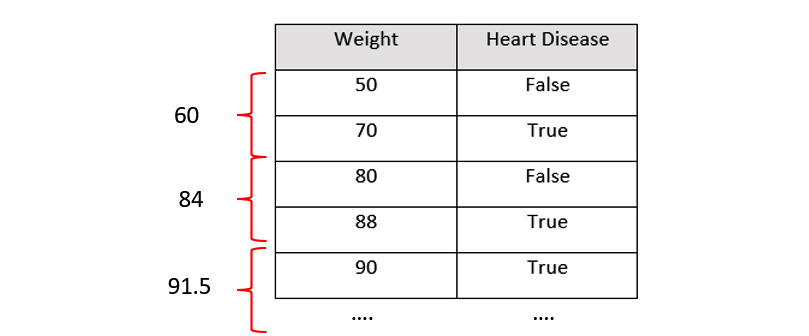
Figure 5.19 – Calculating the average of the subsequent row values

3. Calculate the Gini Impurity of all the averages we calculated:

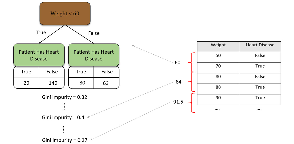
Figure 5.20 – Calculating the Gini Impurity of all the averages

4. Identify and select the average feature value that gives us the least Gini Impurity value.
5. Use the selected feature value as a decision node in the decision tree.

Making predictions using decision trees is very easy. You will have data with values for chest pain, blocked arteries, good circulation, and weight and you will feed it to the decision tree model. The model will filter the values down the decision tree while calculating the node conditions and eventually arriving at the leaf node with the prediction value.

Congratulations – you have just understood the concept of decision trees! Despite decision trees being easy to understand and implement, they are not that good at solving real-life ML problems.

There are certain drawbacks to using decision trees:

• Decision trees are very unstable. Any minor changes in the dataset can drastically alter the performance of the model and prediction results.
• They are inaccurate.
• They can get very complex for large datasets with a large number of features. Imagine a dataset with 1,000 features – the decision tree for this dataset will have a tree whose depth will be very large and its computation will be very resource-intensive.

To mitigate all these drawbacks, the Random Forest algorithm was developed, which builds on top of decision trees. With this knowledge, let’s move on to the next concept: Random Forest.

Introduction to Random Forest

Random Forest, also called Random Decision Forest, is an ML method that builds a large number of decision trees during learning and groups, or ensembles, the results of the individual decision trees to make predictions. Random Forest is used to solve both classification and regression problems. For classification problems, the class value predicted by the majority of the decision trees is the predicted value. For regression problems, the mean or average prediction of the individual trees is calculated and returned as the prediction value.

The Random Forest algorithm follows these steps for learning during training:

1. Create a bootstrapped dataset from the original dataset.
2. Randomly select a subset of the data features.
3. Start creating a decision tree using the selected subset of features, where the feature that splits the data the best is chosen as the root node.
4. Select a random subset of the other remaining features to further split the decision tree.

Let’s understand this concept of Random Forest by creating one.

We shall use the same dataset that we used to make our complex decision tree in Figure 5.17. The dataset is the same one we used to make our decision trees. To create a Random Forest, we need to create a bootstrapped version of the dataset.

A bootstrapped dataset is a dataset that is created from the original dataset by randomly selecting rows from the dataset. The bootstrapped dataset is the same size as the original dataset and can also contain duplicate rows from the original dataset. There are plenty of inbuilt functions for creating a bootstrapped dataset and you can use any of them to create one.

Consider the following bootstrapped dataset:

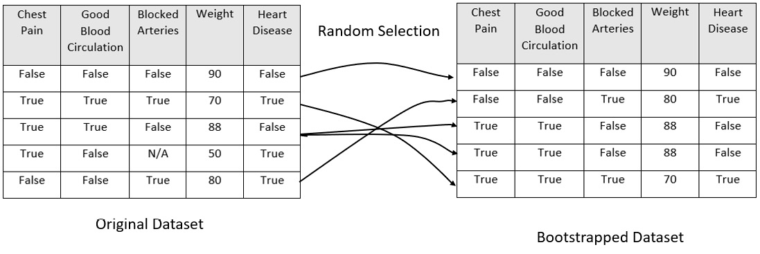
Figure 5.21 – Bootstrapping dataset

The next step is to create a decision tree from the bootstrapped dataset but using only a subset of the feature columns at each step. So, selecting all the features to be considered for the decision tree only lets you go with Good Blood Circulation and Blocked Arteries as features for the decision tree.

We shall follow the same purity identification criteria to determine the root of the node. Let’s assume that for our experiment, Good Blood Circulation is the purest. Setting that as the root node, we shall now consider the remaining features to fill the next level of decision nodes. Just like we did previously, we shall randomly select two features from the remaining features and decide which feature should fit in the next decision node. We will build the tree as usual while considering the random subset of remaining variables at each step.

Here is the tree we just made:

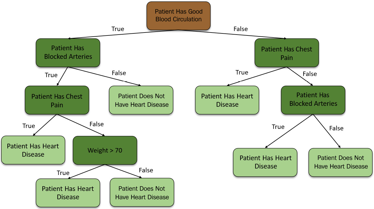
Figure 5.22 – First decision tree from the bootstrapped dataset

Now, we repeat the same process while creating multiple decision trees and bootstrapping and selecting features from random trees. An ideal Random Forest will create hundreds of decision trees, as follows:

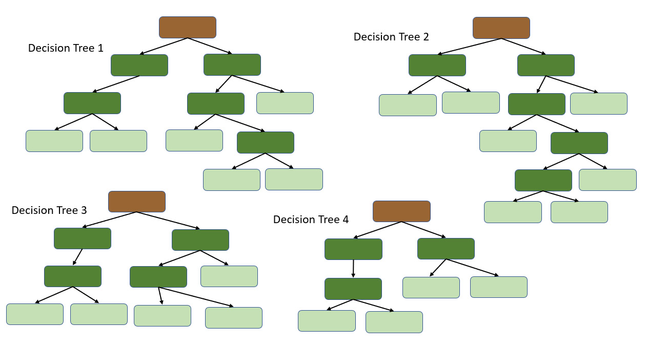
Figure 5.23 – Multiple decision trees from different bootstrapped datasets

This large variety of decision trees that were created with randomized implementation is what makes Random Forest more effective than a single decision tree.

Now that we have created our Random Forest, let’s see how we can use it to make predictions. To make predictions, you will have a row that contains data values for the different features and you want to predict whether that person has heart disease.

You will pass this data down an individual decision tree in the Random Forest:

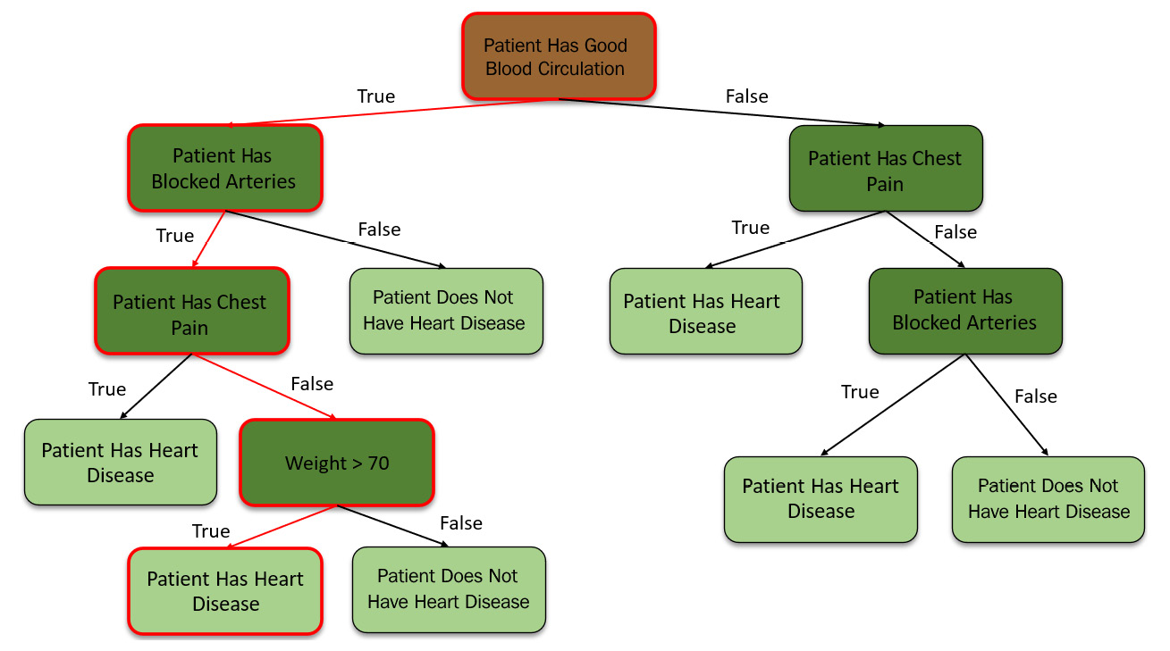
Figure 5.24 – Predictions from the first decision tree in the Random Forest

The decision tree will predict the results based on its structure. We shall keep a track of the prediction made by this tree and continue passing the data down to the other trees, noting their predictions as well:

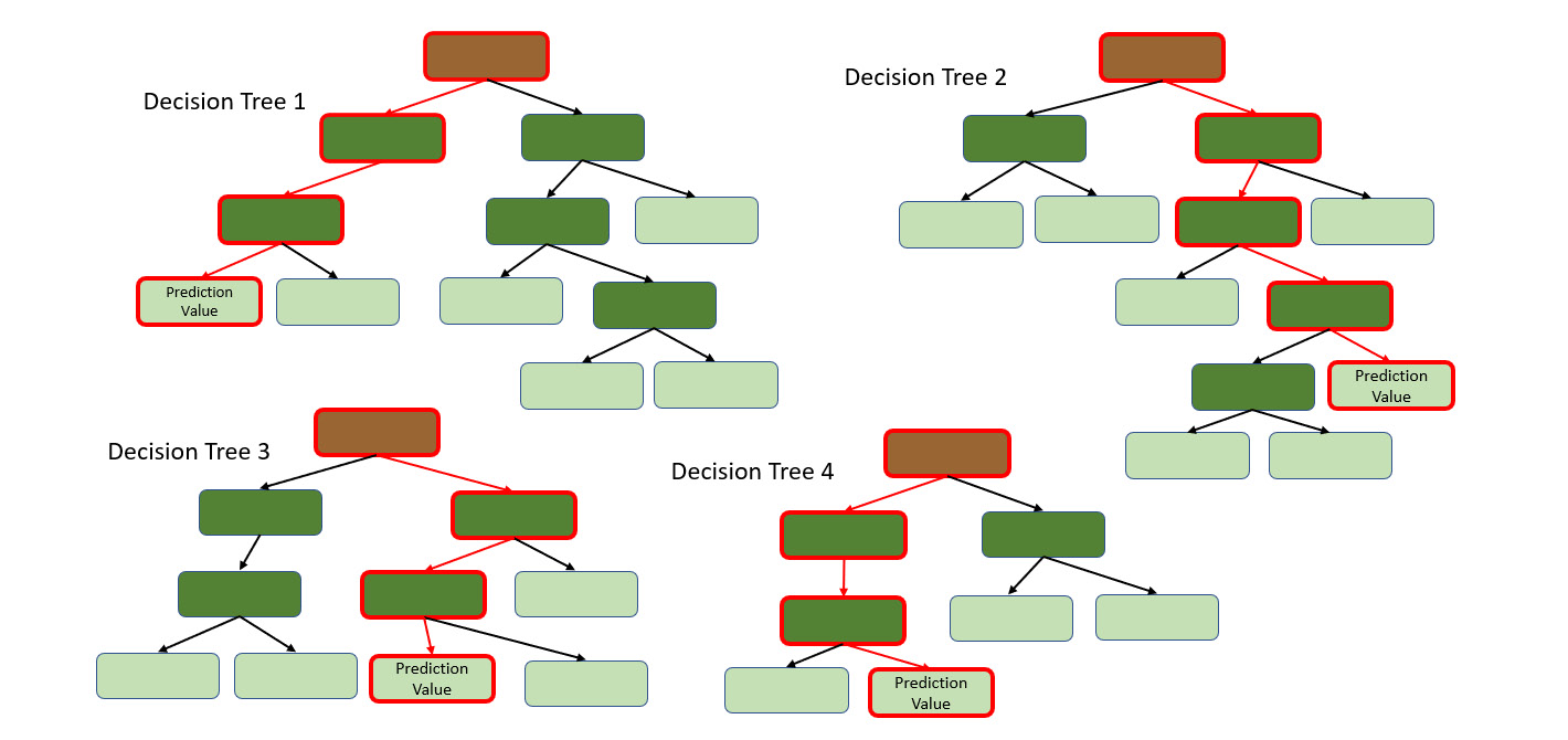
Figure 5.25 – Predictions from the other individual trees in the Random Forest

Once we get predictions from all the individual trees, we can find out which value got the most votes from all the decision trees. The prediction value with the most votes concludes the prediction for the Random Forest.

Bootstrapping the dataset and aggregating the prediction values of all the decision trees to make a decision is called bagging.

Congratulations – you have just understood the concept of Random Forest! Random Forest, despite being a very good ML algorithm with low bias and variance, still suffers from high computation requirements. Hence, H2O AutoML, instead of training Random Forest, trains an alternate version of Random Forest called Extremely Randomized Trees (XRT).

Understanding Extremely Randomized Trees

The XRT algorithm, also called ExtraTrees, is just like the ordinary Random Forest algorithm. However, there are two key differences between Random Forest and XRT, as follows:

• In Random Forest, we use a bootstrapped dataset to train the individual decision trees. In XRT, we use the whole dataset to train the individual decision trees.
• In Random Forest, the decision nodes are split based on certain selection criteria such as the impurity metric or error rate when building the individual decision tree. In XRT, this process is completely randomized and the one with the best results is chosen.

Let’s consider the same example we used to understand Random Forest to understand XRT. We have a dataset, as shown in Figure 5.17. Instead of bootstrapping the data, as we did in Figure 5.20, we shall use the dataset as-is.

Then, we start creating our decision trees by randomly selecting a subset of the features. In Random Forest, we used the purity criteria to decide which feature should be set as the root node of the decision tree. However, for XRT, we shall set the root node as well as the decision nodes of the decision tree randomly. Similarly, we shall create multiple decision trees like these with all the features randomly selected. This added randomness allows the algorithm to further reduce the variance of the model, at the expense of a slight increase in bias.

Congratulations! We have just investigated how the XRT algorithm uses an extremely randomized forest of decision trees to make accurate regressions and classification predictions. Now, let’s understand how the GBM algorithm trains a classification model to classify data.

Understanding the Gradient Boosting Machine algorithm

Gradient Boosting Machine (GBM) is a forward learning ensemble ML algorithm that works on both classification as well as regression. The GBM model is an ensemble model just like the DRF algorithm in the sense that the GBM model, as a whole, is a combination of multiple weak learner models whose results are aggregated and presented as a GBM prediction. GBM works similarly to DRF in that it consists of multiple decision trees that are built in a sequence that sequentially minimizes the error.

GBM can be used to predict continuous numerical values, as well as to classify data. If GBM is used to predict continuous numerical values, we say that we are using GBM for regression. If we are using GBM to classify data, then we say we are using GBM for classification.

The GBM algorithm has a foundation on decision trees, just like DRF. However, how the decision trees are built is different compared to DRF.

Let’s try to understand how the GBM algorithm works for regression.

Building a Gradient Boosting Machine

We shall use the following sample dataset and understand how GBM works as we conceptually build the model. The following table contains a sample of the dataset:

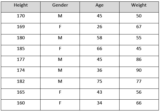
Figure 5.26 – Sample dataset for GBM

This is an arbitrary dataset that we are using just for the sake of understanding how GBM will build its ML model. The contents of the dataset are as follows:

• Height: This column indicates the height of the person in centimeters.
• Gender: This column indicates the gender of the person.
• Age: This column indicates the age of the person.
• Weight: This column indicates the weight of the person.

GBM, unlike DRF, starts creating its weak learner decision trees from leaf nodes instead of root nodes. The very first leaf node that it will create will be the average of all the values of the response variable. So, accordingly, the GBM algorithm will create the leaf node, as shown in the following diagram:

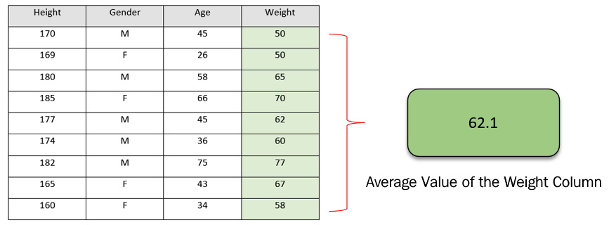
Figure 5.27 – Calculating the leaf node using the column average

This leaf node alone can also be considered a decision tree. It acts like a prediction model that only predicts a constant value for any kind of input data. In this case, it’s the average value that we get from the response column. This is, as we expect, an incorrect way of making any predictions, but it is just the first step for GBM.

The next thing GBM will do is create another decision tree based on the errors it observed from its initial leaf node predictions on the dataset. An error, as we discussed previously, is nothing but the difference between the observed weight and the predicted weight and is also called the residual. However, these residuals are different from the actual residuals that we will get from the complete GBM model. The residuals that we get from the weak learner decision trees of GBM are called pseudo-residuals, while those of the GBM model are the actual residuals.

So, as mentioned previously, the GBM algorithm will calculate the pseudo-residuals of the first leaf node for all the data values in the dataset and create a special column that keeps track of these pseudo-residual values.

Refer to the following diagram for a better understanding:

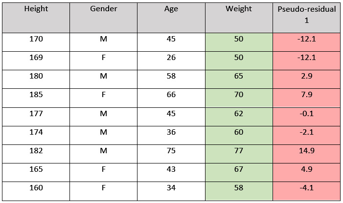
Figure 5.28 – Dataset with pseudo-residuals

Using these pseudo-residual values, the GBM algorithm then builds a decision tree using all the remaining features – that is, Height, Favorite Color, and Gender. The decision tree will look as follows:

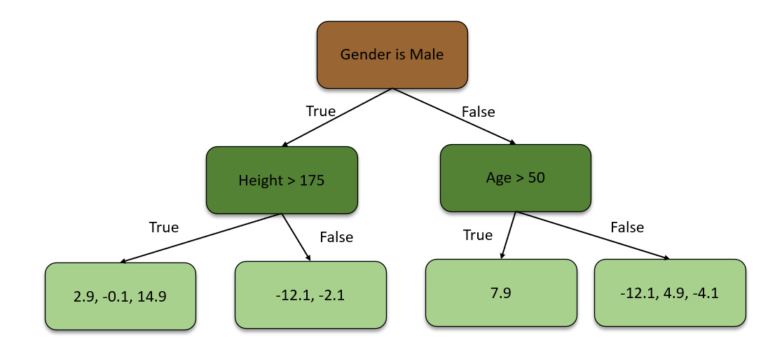
Figure 5.29 – Decision tree using pseudo-residual values

As you can see, this decision tree only has four leaf nodes, while the pseudo-residual values in the algorithm generated from the first tree are way more than four. This is because the GBM algorithm restricts the size of the decision trees it makes. For this scenario, we are only using four leaf nodes. Data scientists can control the size of the trees by passing the right hyperparameters when configuring the GBM algorithm. Ideally, for large datasets, you often use 8 to 32 leaf nodes.

Due to the restriction of the leaf nodes in the decision trees, the decision tree ends up with multiple pseudo-residual values in the same leaf nodes. So, the GBM algorithm replaces them with their average to get one concrete number for a single leaf node. Accordingly, after calculating the averages, we will end up with a decision tree that looks as follows:

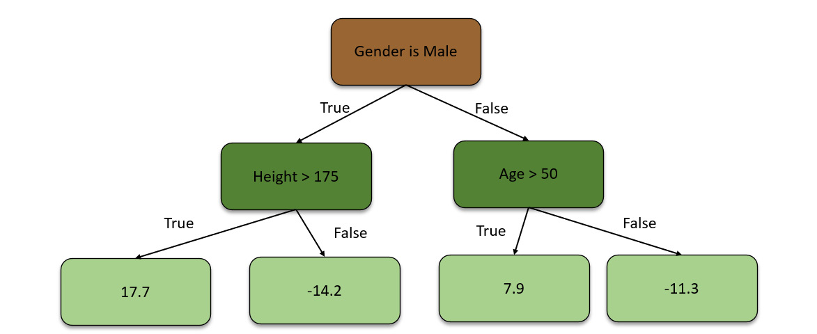
Figure 5.30 – Decision tree using averaged pseudo-residual values

Now, the algorithm combines the original leaf node with this new decision tree to make predictions on it. So, now, we have a value of 71.2 from the initial leaf node prediction. Then, after running the data down the decision tree, we get 16.8. So, the predicted weight is the summation of both the predictions, which is 88. This is also the observed weight.

This is not correct as this is a case of overfitting. Overfitting is a modeling error where the model function is too fine-tuned to predict only the data values available in the dataset and not any other values outside the dataset. As a result, the model becomes useless for predicting any values that fall outside of the dataset.

So, to correct this, the GBM algorithm assigns a learning rate to all the weak learner decision trees that it trains. The learning rate is a hyperparameter that tunes the rate at which the model learns new information that can override the old information. The value of the learning rate ranges from 0 to 1. By adding this learning rate to the predictions from the decision trees, the algorithm controls the influence of the decision tree’s predictions and slowly moves toward minimizing the error step by step. For our example, let’s assume that the learning rate is 0.1. So, accordingly, the predicted weight can be calculated as follows:

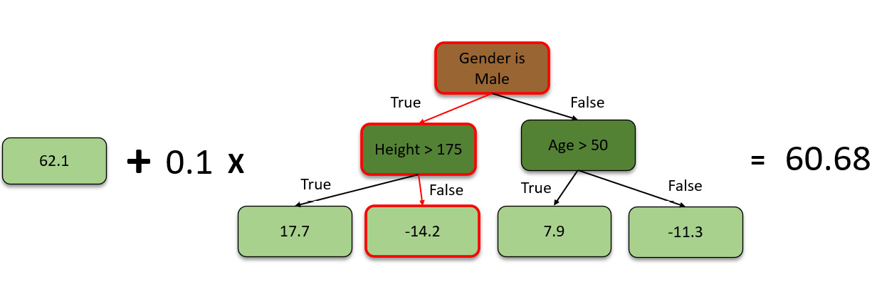
Figure 5.31 – Calculating the predicted weight

Thus, the algorithm will plug in the learning rate for the predictions made by the decision tree and then calculate the predicted weight. Now, the predicted weight will be 62.1 + (0.1 x -14.2) = 60.68.

60.68 is not a very good prediction but it is still a better prediction than 62.68, which is what the initial leaf node predicted. The incremental steps to minimize the errors are the right way to maintain low variance in predictions. A correct balance of learning rate is also important as too high a learning rate will offshoot the correction in the opposite direction, while too low a learning rate will lead to long computation time as the algorithm will take very small correction steps to reach the minimum error.

To further correct the prediction value and minimize the error, the GBM algorithm will create another decision tree. For this, it will calculate the new pseudo-residual values from predictions made with the leaf node and the first decision tree and use these values to build the second decision tree.

The following diagram shows how new pseudo-residual values are calculated:

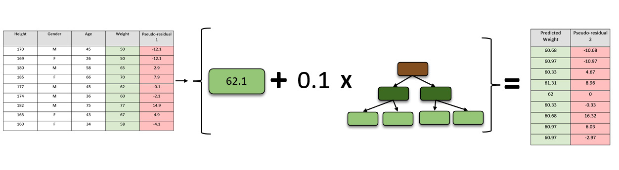
Figure 5.32 – Calculating new pseudo-residual values

You will notice that the new pseudo-residual values that were generated are a lot closer to the actual values compared to the first pseudo-residual values. This indicates that the GBM model is slowly minimizing errors and improving its accuracy.

Moving on with the second decision tree, the algorithm uses the new pseudo residual values to create the second decision tree. Once created, it aggregates the tree, along with the learning rate, to the already existing leaf node and the first decision tree.

The decision trees can be different each time the GBM algorithm creates one. However, the learning rate stays common for all the trees. So, now, the prediction values will be the summation of the three components – the initial leaf node prediction value, the scaled value of the first decision tree prediction, and the scaled value of the second decision tree prediction. So, the prediction values will be as follows:

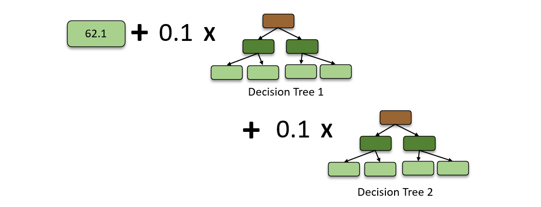
Figure 5.33 – GBM model with a second boosted decision tree

The GBM algorithm will repeat the same process, creating decision trees up to the specified number of trees or until adding decision trees stops improving the predictions. So, eventually, the GBM model will look as follows:

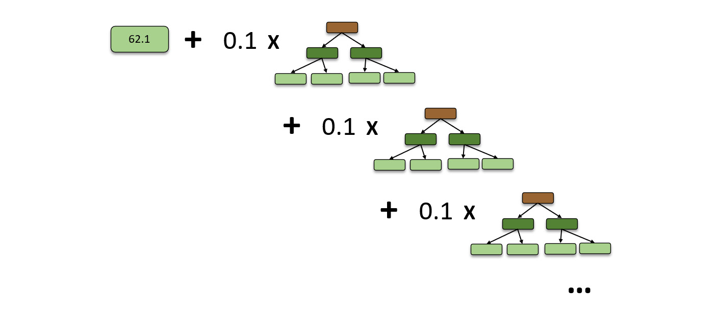
Figure 5.34 – Complete GBM model

Congratulations! we have just explored how the GBM algorithm uses an ensemble of weak decision tree learners to make accurate regressions predictions.

Another algorithm that H2O AutoML uses, which builds on top of GBM, is the XGBoost algorithm. XGBoost stands for Extreme Gradient Boosting and implements a process called boosting that sometimes helps in training better-performing models. It is one of the most widely used ML algorithms in Kaggle competitions and has proven to be an amazing ML algorithm that can be used for both classification and regression. The mathematics behind how XGBoost works can be slightly difficult for users not well versed with statistics. However, it is highly recommended that you take the time and learn more about this algorithm. You can find more information about how H2O performs XGBoost training at https://docs.h2o.ai/h2o/latest-stable/h2o-docs/data-science/xgboost.html.

Tip

Ensemble ML is a method of combining multiple ML models to obtain better prediction results compared to the performance of the models individually – just like how a combination of decision trees creates the Random Forest algorithm using bagging and how the GBM algorithm uses a combination of weak learners to minimize errors. Ensemble models take things one step further by finding the best combinations of prediction algorithms and using their combined performance to train a meta-learner that provides improved performance. This is done using a process called stacking. You can find more information about how H2O trains these stacked ensemble models at https://docs.h2o.ai/h2o/latest-stable/h2o-docs/data-science/stacked-ensembles.html#stacked-ensembles.

Now, let’s learn how deep learning works and understand neural networks.

Understanding what is Deep Learning

Deep Learning (DL) is a branch of ML that develops prediction models using Artificial Neural Networks (ANNs). ANNs, simply called Neural Networks (NNs), are computations that are loosely based on how human brains with neurons work to process information. ANNs consist of neurons, which are types of nodes that are interconnected with other neurons. These neurons transmit information among themselves; this gets processed down the NN to eventually arrive at a result.

DL is one of the most powerful ML techniques and is used to train models that are highly configurable and can support predictions for large and complicated datasets. DL models can be supervised, semi-supervised, or unsupervised, depending on their configuration.

There are various types of ANNs:

• Recurrent Neural Network (RNN): RNN is a type of NN where the connections between the various neurons of the NN can form a directed or undirected graph. This type of network is cyclic since the outputs of the network are fed back to the start of the network and contribute to the next cycle of predictions. The following diagram shows an example of an RNN:

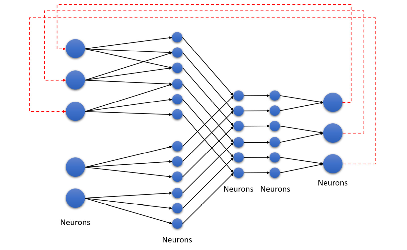
Figure 5.35 – RNN

As you can see, the values from the last nodes in the NN are fed to the starting nodes of the network as inputs.

• Feedforward NN: A feedforward neural network is similar to an RNN, with the only difference being that the network of nodes does not form a cycle. The following diagram shows an example of a feedforward neural network:

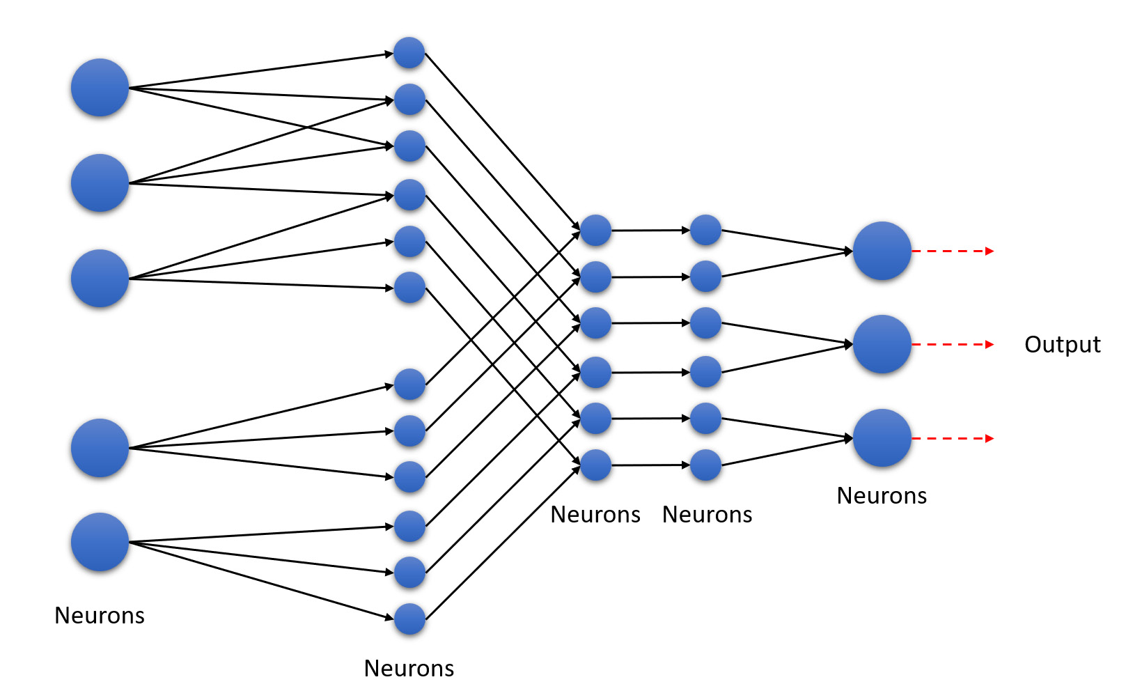
Figure 5.36 – Feedforward neural network

As you can see, this type of NN is unidirectional. This is the simplest type of ANN. A feedforward neural network is also called Deep Neural Network (DNN).

H2O’s DL is based on a multi-layer free forward ANN. It is trained on stochastic gradient descent using backpropagation. There are plenty of different types of DNNs that H2O can train. They are as follows:

• Multi-Layer Perceptron (MLP): These types of DNNs are best suited for tabular data.
• Convolutional Neural Networks (CNNs): These types of DNNs are best suited for image data.
• Recurrent Neural Networks (RNNs): These types of DNNs are best suited for sequential data such as voice data or time series data.

It is recommended to use the default DNNs that H2O provides out of the box as configuring a DNN can be very difficult for non-experts. H2O has already preconfigured its implementation of DL to use the best type of DNNs for the given cases.

With these basics in mind, let’s dive deeper into understanding how DL works.

Understanding neural networks

NNs form the basis of DL. The workings of a NN are easy to understand:

1. You feed the data into the input layer of the NN.
2. The nodes in the NN train themselves to recognize patterns and behaviors from the input data.
3. The NN then makes predictions based on the patterns and behaviors it learns during training.

The structure of an NN looks as follows:

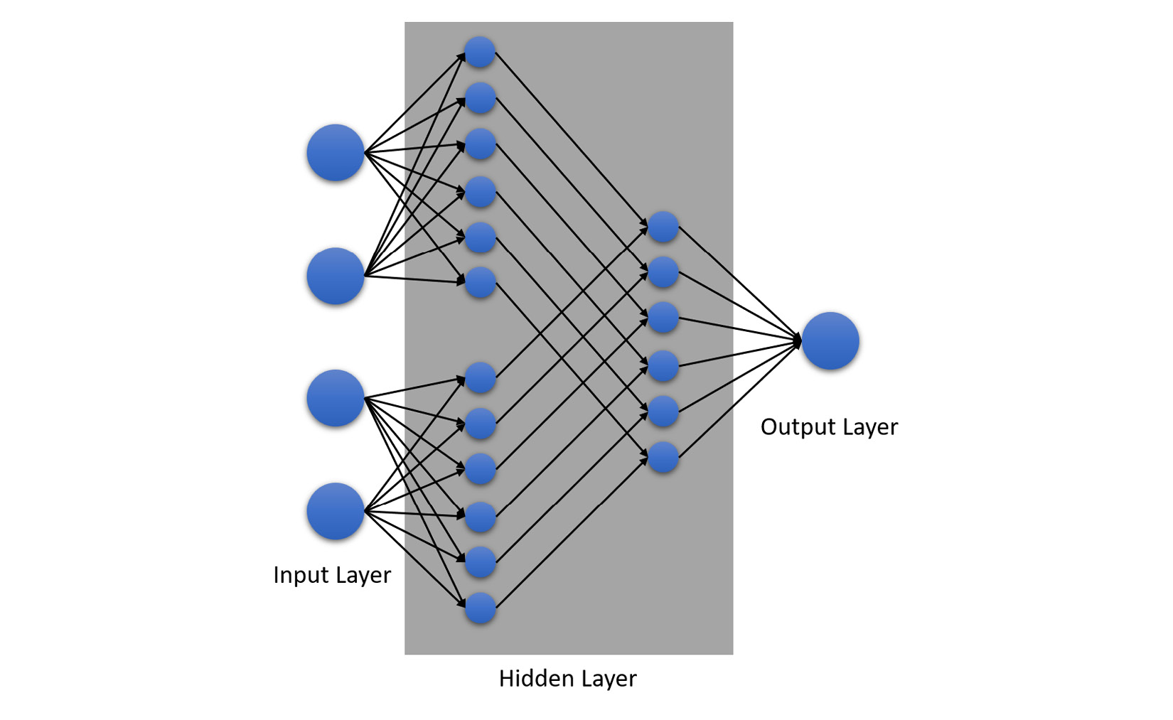
Figure 5.37 – Structure of an NN

There are three essential components of an NN:

• The input layer: The input layer consists of multiple sets of neurons. These neurons are connected to the next layer of neurons, which reside in the hidden layer.
• The hidden layer: Within the hidden layer, there can be multiple layers of neurons, all of which are interconnected layer by layer.
• The output layer: The output layer is the final layer in the NN that makes the final calculations to compute the final prediction values in terms of probability.

The learning process of the NN can be broken down into two components:

• Forward propagation: As the name suggests, forward propagation is where the information flows from the input layer to the output layer through the middle layer. The following diagram shows forward propagation in action:

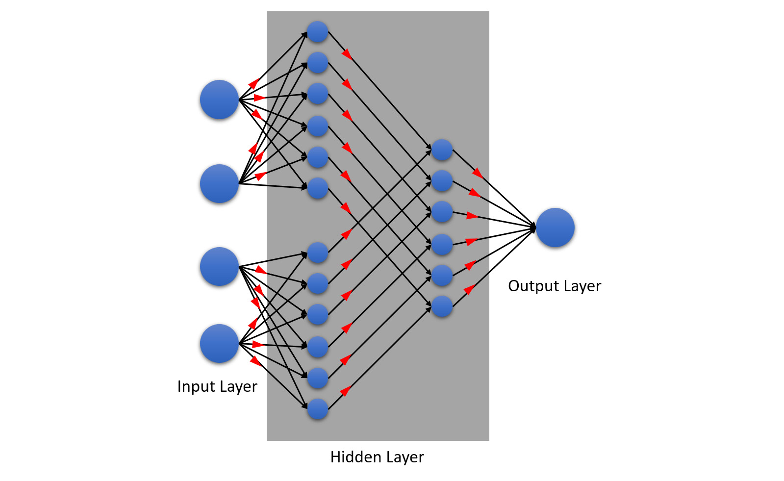
Figure 5.38 – Forward propagation in an NN

The neurons within the middle layer are connected via channels. These channels are assigned numerical values called weights. Weights determine how important the neuron is in terms of its value contributing to the overall prediction. The higher the value of the weight, the more important that node is when making predictions.

The input values from the input layer are multiplied by these weights as they pass through the channels and their sum is sent as inputs to the neurons in the hidden layer. Each neuron in the hidden layer is associated with a numerical value called a bias, which is added to the input sum.

This weighted value is then passed to a non-linear function called the activation function. The activation function is a function that decides if the particular neuron can pass its calculated weight value onto the next layer of the neuron or not, depending on the equation of the non-linear function. The bias is a scalar value that shifts the activation function either to the left or right of the graph for corrections.

This flow of information continues to the next layer of neurons in the hidden layer, following the same process of multiplying the weight of the channels and passing the input to the next activation function of the node.

Finally, in the output layer, the neuron with the highest value determines what the prediction value is, which is a form of probability.

• Backpropagation: Backpropagation works the same way as forward propagation except that it works in the reverse direction. Information is passed from the output layer to the input layer through the hidden layer in a reverse manner. The following diagram will give you a better understanding of this:

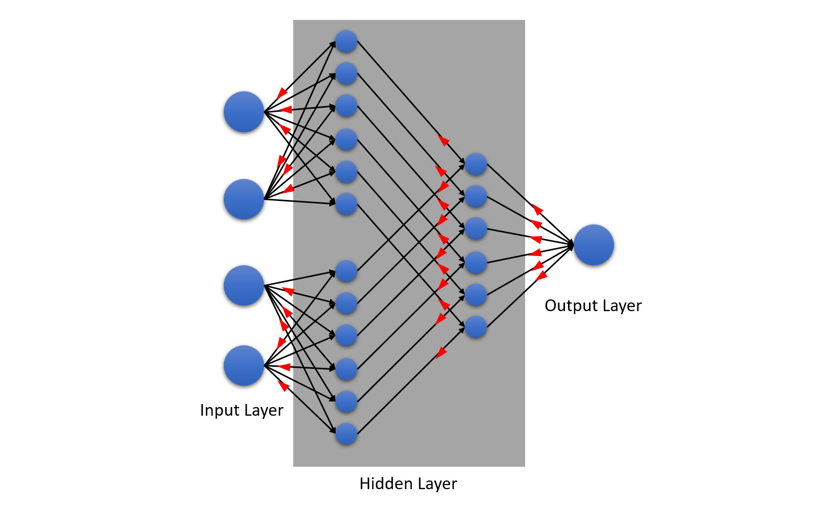
Figure 5.39 – Backpropagation in NN

It may be counterintuitive to understand how backpropagation can work since it works in a reverse manner from the output to the input, but it is a concept that makes DL so powerful for ML. It is through backpropagation that NNs can learn by themselves.

The way it does this is pretty simple. In backpropagation learning, the NN will calculate the magnitude of error between the expected value and the predicted value and evaluate its performance by mapping it onto a loss function. The loss function is a function that calculates the deviance between the predicted and expected values. This deviation value is the information that helps the NN adjust its biases and weights in the hidden layer to improve its performance and make better predictions.

Congratulations – we have just gotten a basic glimpse of how DL trains ML models!

Tip

DL is one of the most sophisticated fields in ML, as well as AI as a whole. It’s a vast area of ML specialization where data scientists spend a lot of time researching and understanding the problem statement and the data they are working with so that they can correctly tune their DL NN. The mathematics behind it is also very complex and as such deserves a dedicated book. So, if you are interested in mathematics and want to excel in the art of DL, feel free to explore the ML algorithm in depth as every step in understanding it will make you that much more of an expert ML engineer. You can find more information about how H2O performs DL training at https://docs.h2o.ai/h2o/latest-stable/h2o-docs/data-science/deep-learning.html.

Summary

In this chapter, we understood the different types of prediction problems and how various algorithms aim to solve them. Then, we understood how the different ML algorithms are categorized into supervised, unsupervised, semi-supervised, and reinforcement based on their method of learning from data. Once we had an understanding of the overall problem domain of ML, we understood that H2O AutoML trains only supervised learning ML algorithms and can solve prediction problems in this domain specifically.

Then, we understood which algorithms H2O AutoML trains starting with GLM. To understand GLM, we understood what linear regression is and how it works and what assumptions about the normal distribution of data it has to make to be effective. With these basics in mind, we understood how GLM is generalized to be effective, even if these assumptions of linear regression are met, which is a common case in real life.

Then, we learned about DRF. To understand DRF, we understood what decision trees are – that is, the basic building blocks of DRF. Then, we learned that multiple decision trees with their ensembled learnings are better ML models than a normal decision tree – that is how Random Forest works. Building on top of this, we learned how DRF adds more randomization in the form of XRT to make the algorithm all the more effective with low variance and bias.

After that, we learned about GBM. We learned how GBM is similar to DRFs but that it has a slightly different way of learning. We understood how GBM sequentially builds decision trees and slowly minimizes error by learning from its residuals from previous decision tree prediction aggregates.

Finally, we learned what DL is. We understood how NNs are the building blocks of DL and their different types. We also understood how NNs perform backpropagation learning from its results and self-learn and improve the model by adjusting the weights and biases of the neurons in the middle layer.

This chapter gave you a brief conceptual understanding of how the various ML algorithms are trained by H2O AutoML without diving too deep into the mathematics. However, ML enthusiasts who want to become experts in the field of ML and wish to work on complex ML problems are strongly encouraged to understand the math behind the wonderful world of ML algorithms. It is the culmination of years of research and effort by scientists and enthusiasts such as yourselves that we have the capability today to potentially predict the future with the help of machines.

In the next chapter, we shall dive deep into understanding how you can understand if an ML model is performing optimally or not using different statistical measurements and other metrics that explain more about ML model performance.