4

Understanding H2O AutoML Architecture and Training

Model training is one of the core components of a Machine Learning (ML) pipeline. It is the step in the pipeline where the system reads and understands the patterns in the dataset. This learning outputs a mathematical representation of the relationship between the different features in the dataset and the target value. The way in which the system reads and analyzes data depends on the ML algorithm being used and its intricacies. This is where the primary complexity of ML lies. Every ML algorithm has its own way of interpreting the data and deriving information from it. Every ML algorithm aims to optimize certain metrics while trading off certain biases and variances. Automation done by H2O AutoML further complicates this concept. Trying to understand how that would work can be overwhelming for many engineers.

Don’t be discouraged by this complexity. All sophisticated systems can be broken down into simple components. Understanding these components and their interaction with each other is what helps us understand the system as a whole. Similarly, in this chapter, we will open up the black box, that is, H2O’s AutoML service, and try to understand what kind of magic makes the automation of ML possible. We shall first understand the architecture of H2O. We shall break it down into simple components and then understand what interaction takes place between the various components of H2O. Later, we will come to understand how H2O AutoML trains so many models and is able to optimize their hyperparameters to get the best possible model.

In this chapter, we are going to cover the following topics:

• Observing the high-level architecture of H2O
• Knowing the flow of interaction between the client and the H2O service
• Understanding how H2O AutoML performs hyperparameter optimization and training

So, let’s begin by first understanding the architecture of H2O.

Observing the high-level architecture of H2O

To deep dive into H2O technology, we first need to understand its high-level architecture. It will not only help us understand what the different software components that make up the H2O AI stack are, but it will also help us understand how the components interact with each other and their dependencies.

With this in mind, let’s have a look at the H2O AI high-level architecture, as shown in the following diagram:

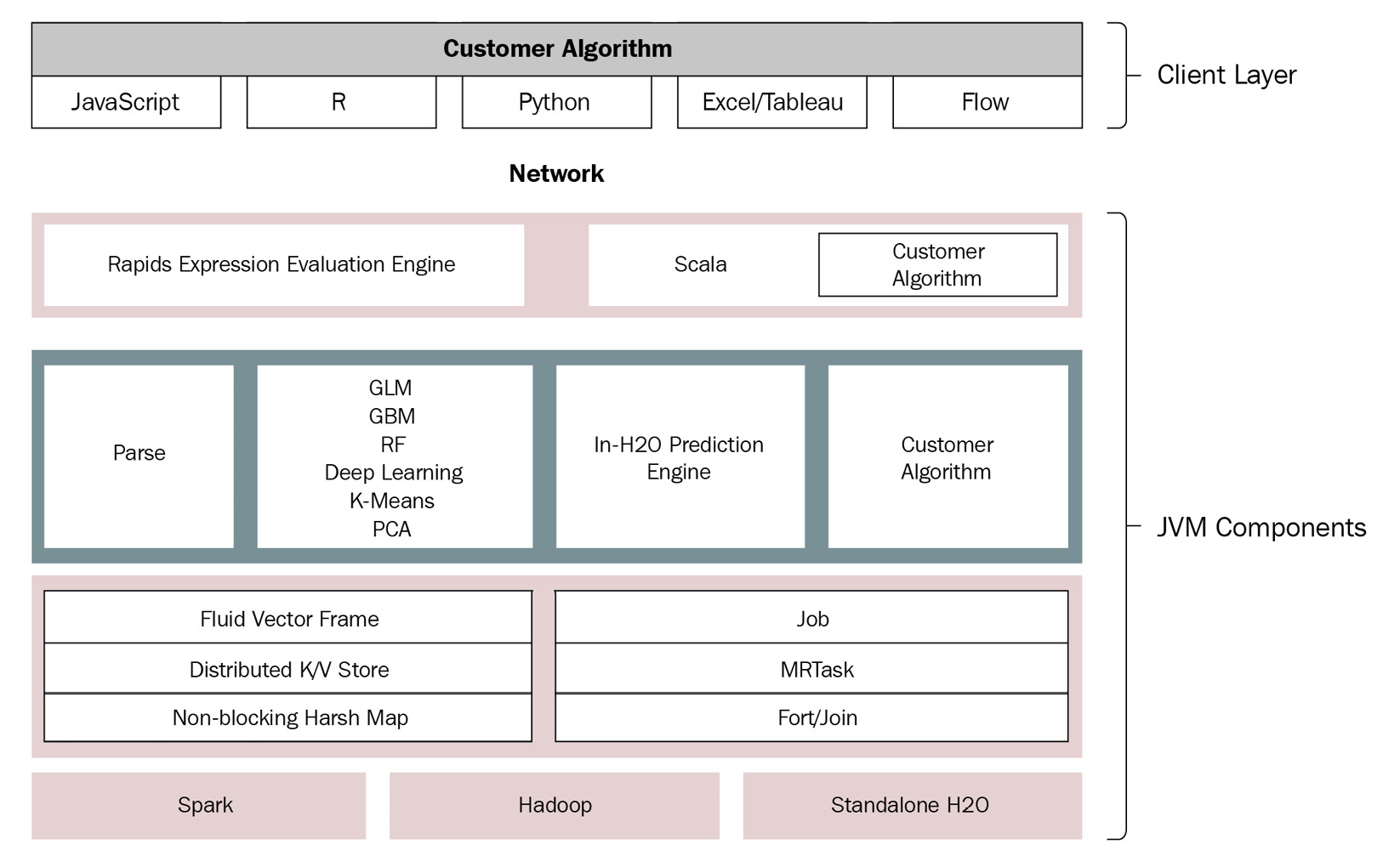
Figure 4.1 – H2O AI high-level architecture

The H2O AI architecture is conceptually divided into two parts, each serving a different purpose in the software stack. The parts are as follows:

• Client layer – This layer points to the client code that communicates with the H2O server.
• Java Virtual Machine (JVM) components – This layer indicates the H2O server and all of its JVM components that are responsible for the different functionalities of H2O AI, including AutoML.

The client and the JVM component layers are separated by the network layer. The network layer is nothing but the general internet, which requests are sent over.

Let’s dive deep into every layer to better understand their functionalities, starting with the first layer, the client layer.

Observing the client layer

The client layer comprises all the client code that you install in your system. You use this software program to send requests to the H2O server to perform your ML activities. The following diagram shows you the client layer from the H2O high-level architecture:

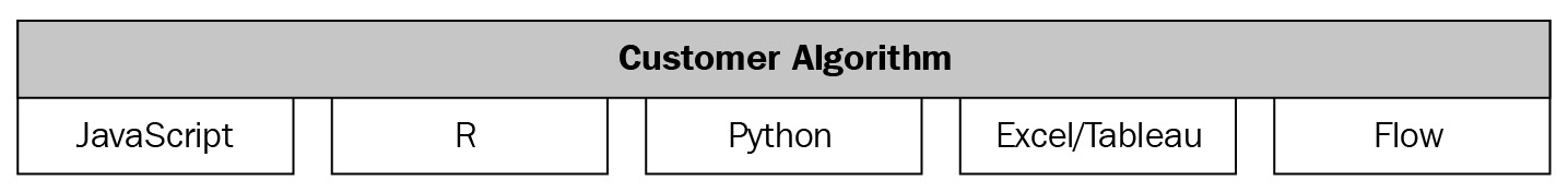
Figure 4.2 – The client layer of H2O high-level architecture

Every supported language will have its own H2O client code that is installed and used in the respective language’s script. All client code internally communicates with the H2O server via a REST API over a socket connection.

The following H2O clients exist for the respective languages:

• JavaScript: H2O’s embedded web UI is written in JavaScript. When you start the H2O server, it starts a JavaScript web client that is hosted on http://localhost:54321. You can log into this client with your web browser and communicate with the H2O server to perform your ML activities. The JavaScript client communicates with the H2O server via a REST API.
• R: Referring to Chapter 1, Understanding H2O AutoML Basics, we import the H2O library by executing library(h2o) and then using the imported H2O variable to import the dataset and train models. This is the R client that is interacting with the initialized H2O server and it does so using a REST API.
• Python: Similarly, in Chapter 1, Understanding H2O AutoML Basics, we import the H2O library in Python by executing import h2o and then using the imported H2O variable to command the H2O server. This is the Python client that is interacting with the H2O server using a REST API.
• Excel: Microsoft Excel is spreadsheet software developed by Microsoft for Windows, macOS, Android, and iOS. H2O has support for Microsoft Excel as well since it is the most widely used spreadsheet software that handles large amounts of two-dimensional data. This data is well suited for analytics and ML. There is an H2O client for Microsoft Excel as well that enables Excel users to use H2O for ML activities through the Excel client.
• Tableau: Tableau is interactive data visualization software that helps data analysts and scientists visualize data in the form of graphs and charts that are interactive in nature. H2O has support for Tableau and, as such, has a dedicated client for Tableau that adds ML capabilities to the data ingested by Tableau.
• Flow: As seen in Chapter 2, Working with H2O Flow (H2O’s Web UI), H2O Flow is H2O’s web user interface that has all the functional capabilities of setting up the entire ML lifecycle in a notebook-style interface. This interface internally runs on JavaScript and similarly communicates with the H2O server via a standard REST API.

The following diagram shows you the interactions of various H2O clients with the same H2O server:

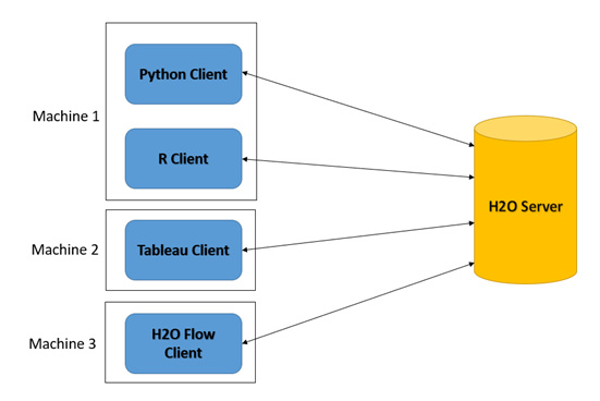
Figure 4.3 – Different clients communicating with the same H2O server

As you can see in the diagram, all the different clients can communicate with the same instance of the H2O server. This enables a single H2O server to service different software products written in different languages.

This covers the contents of the client layer; let’s move down to the next layer in the H2O’s high-level architecture, that is, the JVM component layer.

Observing the JVM component layer

The JVM is a runtime engine that runs Java programs in your system. The H2O cloud server runs on multiple JVM processes, also called JVM nodes. Each JVM node runs specific components of the H2O software stack.

The following diagram shows you the various JVM components that make up the H2O server:

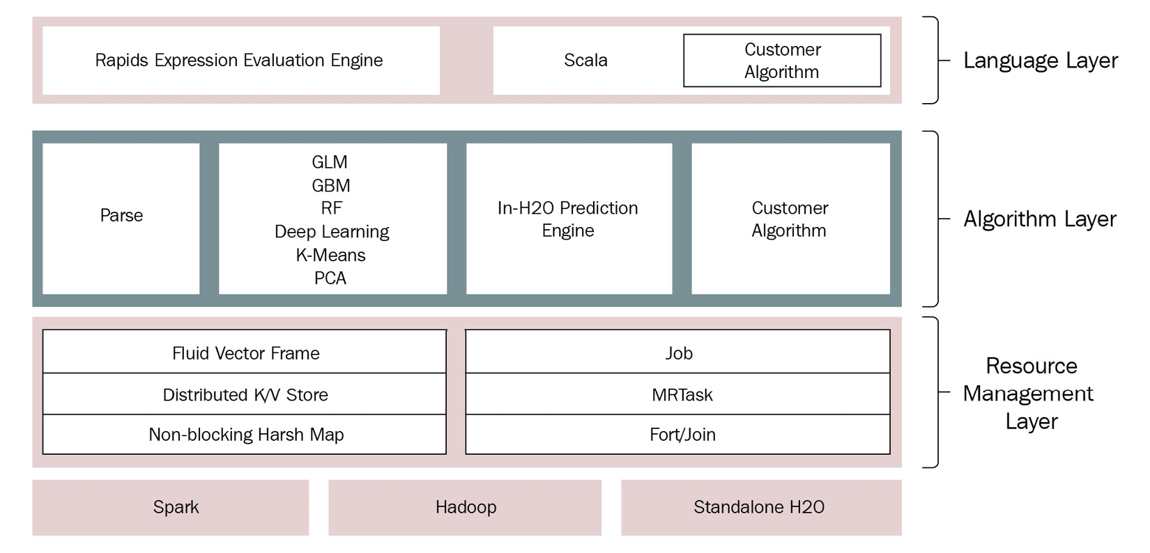
Figure 4.4 – H2O JVM component layer

As seen in the preceding diagram, the JVM nodes are further split into three different layers, which are as follows:

• The language layer: This layer contains processes that are responsible for evaluating the different client language expressions that are sent to the H2O cloud server. The R evaluation layer is a slave to its respective REST client. This layer also contains the Shalala Scala layer. The Shalala Scala library is a code library that accesses dedicated domain-specific language that users can use to write their own programs and algorithms that H2O can use.
• The algorithm layer: This layer contains all the inbuilt ML algorithms that H2O provides. The JVM processes in this layer are responsible for performing all the ML activities, such as importing datasets, parsing, calculating the mathematics for the respective ML algorithms, and overall training of models. This layer also has the prediction engine whose processes perform prediction and scoring functions using the trained models. Any custom algorithms imported into H2O are also housed in this layer and the JVM processes handle the execution just like the other algorithms.
• The resource management layer: This layer contains all the JVM processes responsible for the efficient management of system resources such as memory and CPU when performing ML activities.

Some of the JVM processes in this layer are as follows:

• Fluid Vector frame: A frame, also called a DataFrame, is the basic data storage object in H2O. Fluid Vector is a term coined by engineers at H2O.ai that points to the efficient (or, in other words, fluid) way by which the columns in the DataFrame can be added, updated, or deleted, as compared to the DataFrames in the data engineering domain, where they are usually said to be immutable in nature.
• Distributed key-value store: A key-value store or database is a data storage system that is designed to retrieve data or values efficiently and quickly from a distributed storage system using indexed keys. H2O uses this distributed key-value in-memory storage across its cluster for quick storage and lookups.
• NonBlockingHashMap: Usually in a database to provide Atomicity, Consistency, Isolation, and Durability (ACID) properties, locking is used to lock data when updates are being performed on it. This stops multiple processes from accessing the same resource. H2O uses a NonBlockingHashMap, which is an implementation of ConcurrentHashMap with better scaling capabilities.
• Job: In programming, a job is nothing but a large piece of work that is done by software that serves a single purpose. H2O uses a jobs manager that orchestrates various jobs that perform complex tasks such as mathematical computations with increased efficiency and less CPU resource consumption.
• MRTask: H2O uses its own in-memory MapReduce task to perform its ML activities. MapReduce is a programming model that is used to process large amounts of computation or data read and writes using parallel execution of tasks on a distributed cluster. MapReduce helps the system perform computational activities faster than sequential computing.
• Fork/Join: H2O uses a modified Java concurrency library called jsr166y to perform the concurrent execution of tasks. jsr166y is a very lightweight task execution framework that uses Fork, where the process breaks down a task into smaller subtasks, and Join, where the process joins the results of the subtasks together to get the final output of the task.

The entire JVM component layer lies on top of Spark and Hadoop data processing systems. The components in the JVM layer leverage these data processing cluster management engines to support cluster computing.

This sums up the entire high-level architecture of H2O’s software technology. With this background in mind, let’s move to the next section, where we shall understand the flow of interaction between the client and H2O and how the client-server interaction helps us perform ML activities.

Learning about the flow of interaction between the client and the H2O service

In Chapter 1, Understanding H2O AutoML Basics, and Chapter 2, Working with H2O Flow (H2O’s Web UI), we saw how we can send a command to H2O to import a dataset or train a model. Let’s try to understand what happens behind the scenes when you send a request to the H2O server, beginning with data ingestion.

Learning about H2O client-server interactions during the ingestion of data

The process of a system ingesting data is the same as how we read a book in real life: we open the book and start reading one line at a time. Similarly, when you want your program to read a dataset stored in your system, you will first inform the program about the location of the dataset. The program will then open the file and start reading the bytes of the data line by line and store it in its RAM. However, the issue with the type of sequential data reading in ML is that datasets tend to be huge in ML. Such data is often termed big data and can span from gigabytes to terabytes of volume. Reading such huge volumes of data by a system, no matter how fast it may be, will need a significant amount of time. This is time that ML pipelines do not have, as the aim of an ML pipeline is to make predictions. These predictions won’t have any value if the time to make decisions has already passed. For example, if you design an ML system that is installed in a car that automatically stops the car if it detects a possibility of collision, then the ML system would be useless if it spent all its time reading data and was too late to make collision predictions before they happened.

This is where parallel computing or cluster computing comes in. A cluster is nothing but multiple processes connected together over a network that performs like a single entity. The main aim of cluster computing is to parallelize long-running sequential tasks using these multiple processes to finish the task quickly. It is for this reason that cluster computing plays a very important role in ML pipelines. H2O also rightly uses clusters to ingest data.

Let’s observe how a data ingestion interaction request flows from the H2O client to the H2O server and how H2O ingests data.

Refer to the following diagram to understand the flow of data ingestion interaction:

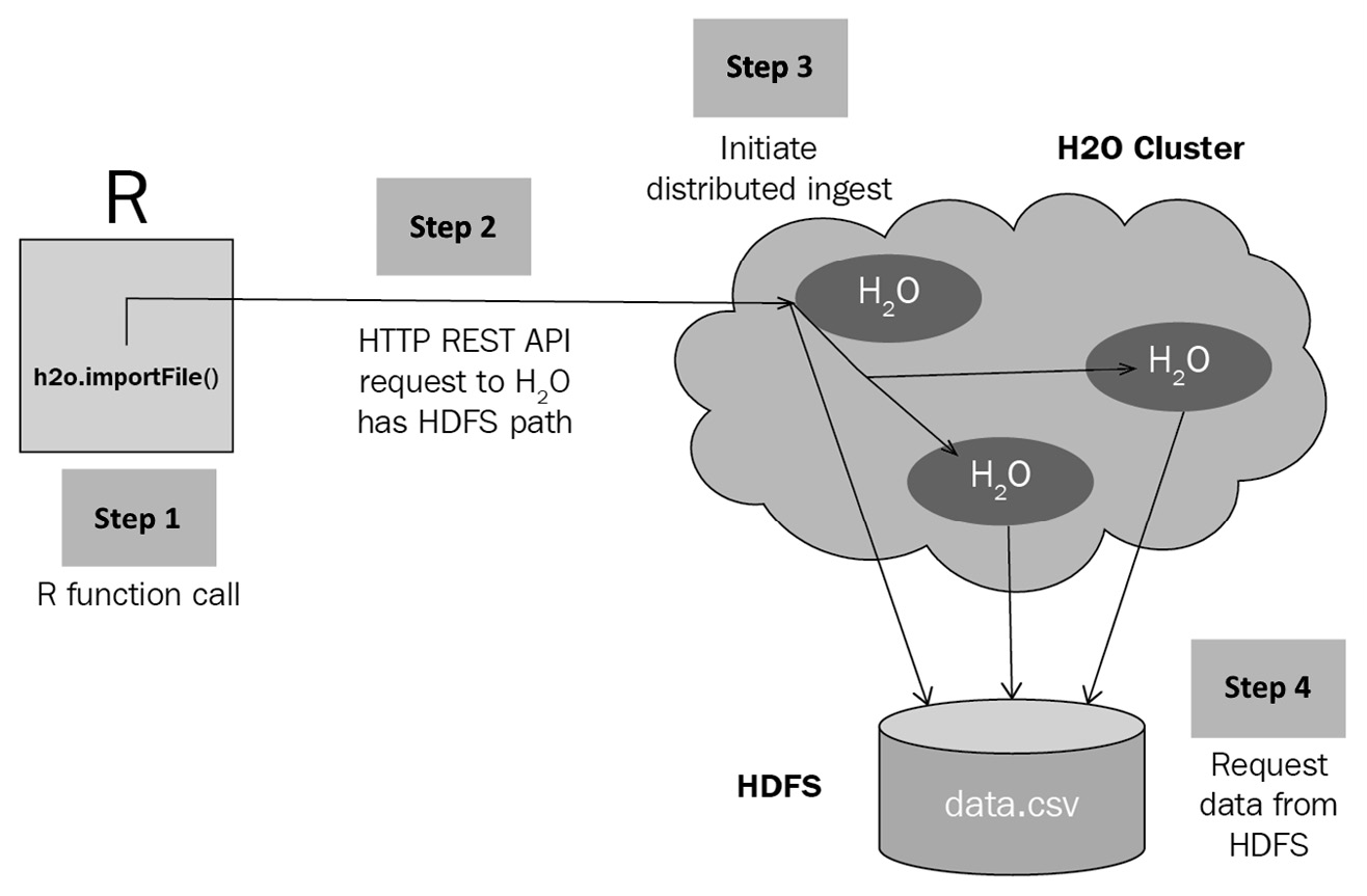
Figure 4.5 – H2O data ingestion request interaction flow

The following sequence of steps describes how a client request to the H2O cluster server to ingest data is serviced by H2O using the Hadoop Distributed File System (HDFS):

1. Making the request: Once the H2O cluster server is up and running, the user using the H2O client makes a data ingestion function call pointing to the location of the dataset (see Step 1 in Figure 4.5). The function call in Python would be as follows:

   h2o.import_file("Dataset/iris.data")

The H2O client will extract the dataset location from the function call and internally create a REST API request (see Step 2 in Figure 4.5). The client will then send the request over the network to the IP address where the H2O server is hosted.

2. H2O server processing the request: Once the H2O cluster server receives the HTTP request from the client, it will extract the dataset location path value from the request and initiate the distributed dataset ingestion process (see Step 3 in Figure 4.5). The cluster nodes will then coordinate and parallelize the task of reading the dataset from the given path (see Step 4 in Figure 4.5).

Each node will read a section of the dataset and store it in its cluster memory.

3. Ingestion of data: The data read from the dataset location path will be stored in blocks in the distributed H2OFrame cluster memory (see Step 1 in Figure 4.6). The block of data is stored in a distributed key-value store (see Step 2 in Figure 4.6). Once the data is fully ingested, the H2O server will create a pointer that points to the ingested dataset stored in the key-value store and return it to the requesting client (see Step 3 in Figure 4.6).

Refer to the following diagram to understand the flow of interaction once data is ingested and H2O returns a response:

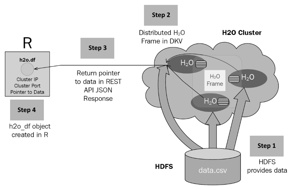
Figure 4.6 – H2O data ingestion response interaction flow

Once the client receives the response, it creates a DataFrame object that contains this pointer, which the user can then later use to run any further executions on the ingested dataset (see Step 4 in Figure 4.6). In this way, with the use of pointers and the distributed key-value store, H2O can work on DataFrame manipulations and usage without needing to transfer the huge volume of data that it ingested between the server and client.

Now that we understand how H2O ingests data, let us now look into how it handles model training requests.

Knowing the sequence of interactions in H2O during model training

During model training, there are plenty of interactions that take place, right from the users making the model training request to the user getting the trained ML model. The various components of H2O perform the model training activity using a series of coordinated messages and scheduled jobs.

To better understand what happens internally when a model training request is sent to the H2O server, we need to dive deep into the sequence of interactions that occur during model training.

We shall understand the sequences of interactions by categorizing them as follows:

1. The client starts a model training job.
2. H2O runs the model training job.
3. The client polls for job completion status.
4. The client queries for the model information.

So, let’s begin first by understanding what happens when the client starts a model training job.

The client starts a model training job

The model training job starts when the client first sends a model training request to H2O.

The following sequence diagram shows you the sequence of interactions that take place inside H2O when a client sends a model training request:

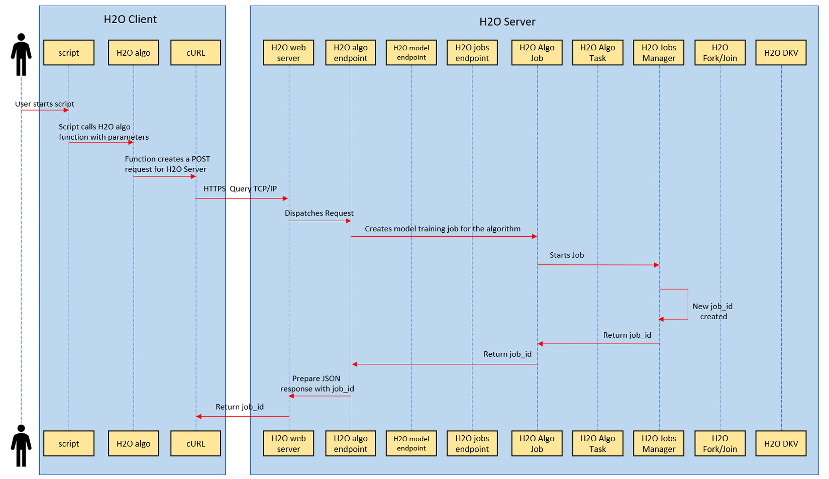
Figure 4.7 – Sequence of interactions in the model training request

The following set of sequences takes place during a model training request:

1. The user first runs a script that contains all the instructions and function calls to make a model training request to H2O.
2. The script contains a model training function call with its respective parameters. This also includes an H2O AutoML function call that performs in a similar manner.
3. The function call instructs the respective language-specific H2O client, which creates a POST request that contains all the parametric information needed to train the model correctly.
4. The H2O client will then perform a curl operation that sends the HTTP POST request to the H2O web server at the host IP address that it is hosted on.
5. From this point onward, the flow of information is performed inside the H2O server. The H2O server dispatches the request to the appropriate model training endpoint based on the model that was chosen to be trained by the user.
6. This model training endpoint extracts the parameter values from the request and schedules a job.
7. The job, once scheduled, starts training the model.
8. The job manager is responsible for handling all the jobs that are currently in progress, as well as allocating resources and scheduling. The job manager will create a unique job_id for the training job, which can be used to identify the progress of the job.
9. The job manager then sends the job_id back to the training job, which assigns it to itself.
10. The training job in turn returns the same job_id to the model training endpoint.
11. The model training endpoint creates a JSON response that contains this job_id and instructs the web server to send it back as a response to the client making the request.
12. The web server accordingly makes an HTTP response that transfers over the network and reaches the H2O client.
13. The client then creates a model object that contains this job_id, which the user can further use to track the progress of the model training or perform predictions once training is finished.

This sums up the sequence of events that take place inside the H2O server when it receives a model training request.

Now that we understand what happens to the training request, let’s understand what the events that take place are when the training job created in step 6 is training the model.

H2O runs the model training job

In H2O, the training of a model is carried out by an internal model training job that acts independently from the user’s API request. The user’s API request just initiates the job; the job manager does the actual execution of the job.

The following sequence diagram shows you the sequence of interactions that take place when a model training job is training a model:

Figure 4.8 – Sequence of interactions in the model training job execution

The following set of sequences takes place during model training:

1. The model training job breaks down the model training into tasks.
2. The job then submits the tasks to the execution framework.
3. The execution framework uses the Java concurrency library jsr166y to perform the task in a concurrent manner using the Fork/Join processing framework.
4. Once a forked task is successfully executed, the execution library sends back the completed task results.
5. Once all the tasks are completed, the model that is trained is sent back to the model training job.
6. The model training job then stores the model object in H2O’s distributed key-value storage and tags it with a unique model ID.
7. The training job then informs the job manager that model training is completed and the job manager is then free to move on to other training jobs.

Now that we understand what goes on behind the scenes when a model training job is training a model, let’s move on to understand what happens when a client polls for the model training status.

Client polls for model training job completion status

As mentioned previously, the actual training of the model is processed independently from the client’s training request. In this case, once a training request is sent by the client, the client is in fact unaware of the progress of the model. The client will need to constantly poll for the status of the model training job. This could be done either via manually making a request using HTTP or via certain client software features, such as progress trackers polling the H2O server for the status of the model training at regular intervals.

The following sequence diagram shows you the sequence of interactions that takes place when a client polls for the model training job completion:

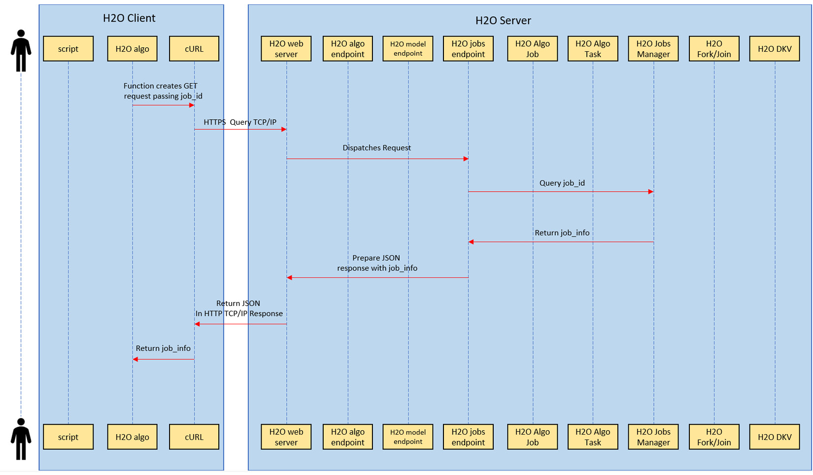
Figure 4.9 – User polling for the model status sequence of interactions

The following set of sequences takes place when the client polls for the model training job completion:

1. To get the status of the model training, the client will make a GET request, passing the job_id that it received as a response when it first made a request to train a model.
2. The GET request transfers over the network and to the H2O web server at the host IP address.
3. The H2O web server dispatches the request to the H2O jobs endpoint.
4. The H2O jobs endpoint will then query the jobs manager, requesting the status of the job_id that was passed in the GET request.
5. The job manager will return the job info of the respective job_id that contains information about the progress of the model training.
6. The H2O jobs endpoint will prepare a JSON response containing the job information for the job_id and send it to the H2O web server.
7. The H2O web server will in turn send the JSON as a response back to the client making the request.
8. Upon receiving the response, the client will unpack this JSON and update the user about the status of the model training based on the job information.

This sums up the various interactions that take place when a client polls for the status of model training. With this in mind, let’s now see what happens when a client requests for the model info once it is informed that the model training job has finished training the model.

Client queries for model information

Once a model is trained successfully, the user will most likely want to analyze the details of the model. An ML model has plenty of metadata associated with its performance and quality. This metadata is very useful even before a model is used for predictions. But as we saw in the previous section, the model training process was independent of the user’s request, and H2O did not return a model object once training was complete. However, the H2O server does provide an API, using which you can get the information about a model already stored in the server.

The following sequence diagram shows you the sequence of interactions that take place when a client requests information about a trained model:

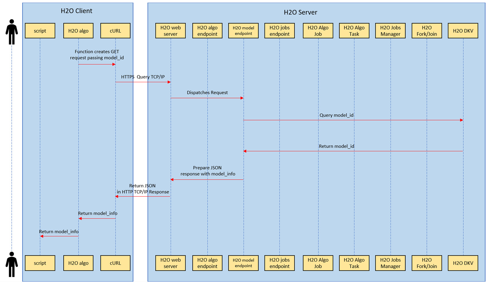
Figure 4.10 – User querying for model information

The following set of sequences takes place when the client polls for the model training job completion:

1. To get the model information, the client will make a GET request passing the unique model_id of the ML model.
2. The GET request transfers over the network and to the H2O web server at the host IP address.
3. The H2O web server dispatches the request to the H2O model endpoint.
4. All the model information is stored in H2O’s distributed key-value storage when the model training job finishes training the model. The H2O model endpoint will query this distributed key-value storage with the model_id as the filter.
5. The distributed key-value storage will return all the model information for the model_id passed to it.
6. The H2O model endpoint will then prepare a JSON response containing the model information and send it to the H2O web server.
7. The H2O web server will in turn send the JSON as a response back to the client making the request.
8. Upon receiving the response, the client will extract all the model information and display it to the user.

A model, once trained, is stored directly in the H2O server itself for quick access whenever there are any prediction requests. You can download the H2O model as well; however, any model not imported into the H2O server cannot be used for predictions.

This sums up the entire sequence of interactions that takes place in various parts of the H2O client-server communication. Now that we understand how H2O trains models internally using jobs and the job manager, let’s dive deeper and try to understand what happens when H2O AutoML trains and optimizes hyperparameters, eventually selecting the best model.

Understanding how H2O AutoML performs hyperparameter optimization and training

Throughout the course of this book, we have marveled at how the AutoML process automates the sophisticated task of training and selecting the best model without us needing to lift a finger. Behind every automation, however, there is a series of simple steps that is executed in a sequential manner.

Now that we have a good understanding of H2O’s architecture and how to use H2O AutoML to train models, we are now ready to finally open the black box, that is, H2O AutoML. In this section, we shall understand what H2O AutoML does behind the scenes so that it automates the entire process of training and selecting the best ML models.

The answer to this question is pretty simple. H2O AutoML automates the entire ML process using grid search hyperparameter optimization.

Grid search hyperparameter optimization sounds very intimidating to a lot of non-experts, but the concept in itself is actually very easy to understand, provided that you know some of the basic concepts in model training, especially the importance of hyperparameters.

So, before we dive into grid search hyperparameter optimization, let’s first come to understand what hyperparameters are.

Understanding hyperparameters

Most software engineers are aware of what parameters are: certain variables containing certain user input data, or any system-calculated data that is fed to another function or process. In ML, however, this concept is slightly complicated due to the introduction of hyperparameters. In the field of ML, there are two types of parameters. One type we call the model parameters, or just parameters, and the other is hyperparameters. Even though they have a similar name, there are some important differences between them that all software engineers should keep in mind when working in the ML space.

So, let’s understand them by simple definition:

• Model parameters: A model parameter is a parameter value that is calculated or learned by the ML algorithm from the given dataset during model training. Some examples of basic model parameters are mean or standard deviation, weights, and biases of data in the dataset. These are elements that we learn from the training data when we are training the model and these are the parametric values that the ML algorithm uses to train the ML model. Model parameters are also called internal parameters. Model parameters are not adjustable in a given ML training scenario.
• Hyperparameters: Hyperparameters are configurations that are external to the model training and are not derived from the training dataset. These are parametric values that are set by the ML practitioner and are used to derive the model parameters. They are values that are heuristically discovered by the ML practitioner and input to the ML algorithm before model training begins. Some simple examples of hyperparameters are the number of trees in a random forest, or the learning rate in regression algorithms. Every type of ML algorithm will have its own required set of hyperparameters. Hyperparameters are adjustable and are often experimented with to get the optimal model in a given ML training scenario.

The aim of training an optimal model is simple:

1. You select the best combination of hyperparameters.
2. These hyperparameters generate the ideal model parameters.
3. These model parameters train a model with the lowest possible error rate.

Sounds simple enough. However, there is a catch. Hyperparameters are not intuitive in nature. One cannot simply just observe the data and decide x value for the hyperparameter will get us the best model. Finding the perfect hyperparameter is a trial-and-error process, where the aim is to find a combination that minimizes errors.

Now, the next question that arises is how you find the best hyperparameters for training a model. This is where hyperparameter optimization comes into the picture, which we will cover next.

Understanding hyperparameter optimization

Hyperparameter optimization, also known as hyperparameter tuning, is the process of choosing the best set of hyperparameters for a given ML algorithm to train the most optimal model. The best combination of these values minimizes a predefined loss function of an ML algorithm. A loss function in simple terms is a function that measures some unit of error. The loss function is different for different ML algorithms. A model with the lowest possible amount of errors among a potential combination of hyperparameter values is said to have optimal hyperparameters.

There are many approaches to implementing hyperparameter optimization. Some of the most common ones are grid search, random grid search, Bayesian optimization, and gradient-based optimization. Each is a very broad topic to cover; however, for this chapter, we shall focus on only two approaches: grid search and random grid search.

Tip

If you want to explore more about the Bayesian optimization technique for hyperparameter tuning, then feel free to do so. You can get additional information on the topic at this link: https://arxiv.org/abs/1807.02811. Similarly, you can get more details on gradient-based optimization at this link: https://arxiv.org/abs/1502.03492.

It is actually the random grid search approach that is used by H2O’s AutoML for hyperparameter optimization, but you need to have an understanding of the original grid search approach to optimization in order to understand random grid search.

So, let’s begin with grid search hyperparameter optimization.

Understanding grid search optimization

Let’s take the example of the Iris Flower Dataset that we used in Chapter 1, Understanding H2O AutoML Basics. In this dataset, we are training a model that is learning from the sepal width, sepal length, petal width, and petal length to predict the classification type of the flower.

Now, the first question you are faced with is: which ML algorithm should be used to train a model? Assuming you do come up with an answer to that and choose an algorithm, the next question you will have is: which combination of hyperparameters will get me the optimal model?

Traditionally, ML practitioners would train multiple models for a given ML algorithm with different combinations of hyperparameter values. They would then compare the performance of these models and find out which hyperparameter combination trained the model with the lowest possible error rate.

The following diagram shows you how different combinations of hyperparameters train different models with varying performance:

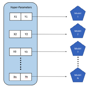
Figure 4.11 – Manual hyperparameter tuning

Let’s take an example where you are training a decision tree. Its hyperparameters are the number of trees, ntrees, and the maximum depth, max_depth. If you are performing a manual search for hyperparameter optimization, then you will initially start out with values like 50, 100, 150, and 200 for ntrees and 5, 10, and 50 for max_depth, train the models, and measure their performance. When you find out which combination of those values gives you the best results, you set those values as the threshold and tweak them with smaller increments or decrements, retrain the models with these new hyperparameter values, and compare the performance again. You keep doing this until you find the best set of hyperparameter values that gives you the optimum performance.

This method, however, has a few drawbacks. Firstly, the range of values you can try out initially is limited since you can only train so many models manually. So, if you have a hyperparameter whose value can range between 1 and 10,000, then you need to make sure that you cover enough ground to not miss the ideal value by a huge margin. If you do, then you will end up constantly tweaking the value with smaller increments or decrements, spending lots of time optimizing. Secondly, as the number of hyperparameters increases and the number of possible values and combinations of values you want to use increases, it becomes tedious for the ML practitioner to manage and run optimization processes.

To manage and partially automate this process of training multiple models with different hyperparameters, grid search was invented. Grid search is also known as Cartesian Hyperparameter Search or exhaustive search.

Grid search basically maps all the values for given hyperparameters over a Cartesian grid and exhaustively searches combinations in the grid to train models. Refer to the following diagram, which shows you how a hyperparameter grid search translates to multiple models being trained:

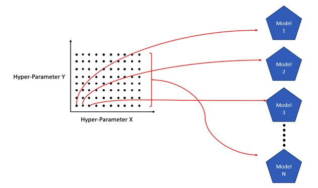
Figure 4.12 – Cartesian grid search hyperparameter tuning

In the diagram, we can see that we have a two-dimensional grid that maps the two hyperparameters. Using this Cartesian grid, we can further expand the combination of hyperparameter values to 10 values per parameter, extending our search. The grid search approach exhaustively searches across different values of the two hyperparameters. So, it will have 100 different combinations and will train 100 different models in total, all trained without needing much manual intervention.

H2O does have grid search capabilities that users can use to test out their own manually implemented grid search approach for hyperparameter optimization. When training models using grid search, H2O will map all models that it trains to the respective hyperparameter value combinations of the grid. H2O also allows you to sort all these models based on any supported model performance metrics. This sorting helps you quickly find the best-performing model based on the metric values. We shall explore more about performance metrics in Chapter 6, Understanding H2O AutoML Leaderboard and Other Performance Metrics.

However, despite automating and introducing a quality-of-life improvement to manual searching, there are still some drawbacks to this approach. Grid search hyperparameter optimization suffers from what is called the curse of dimensionality.

The curse of dimensionality was a term coined by Richard E. Bellman when considering problems in dynamic programming. From the point of view of ML, this concept states that as the number of hyperparameter combinations increases, the number of evaluations that the grid search will perform increases exponentially.

For example, let’s say you have a hyperparameter x and you want to try out integer values 1-20. In this case, you will end up doing 20 evaluations, in other words, training 20 models. Now suppose that there is another hyperparameter y and you want to try out the values 1-20 in combination with the values for x. Your combinations will be as follows:

(1,1), (1,2), (1,3), (1,4), (1,5), (1,6), (1,7)….(20,20) where (x, y)

Now, there are 20x20=400 combinations in total in your grid, for which your grid search optimization will end up training 400 models. Add another hyperparameter z to it and your number of combinations will skyrocket beyond management. The more hyperparameters you have, the more combinations you would try and the more combinatorial explosion will occur.

Given the time and resource sensitivity of ML, an exhaustive search is counterproductive to finding the best model. The real world has limitations, hence a random selection of hyperparameter values has often been proven to provide better results than an exhaustive grid search.

This brings us to our next approach in hyperparameter optimization, random grid search.

Understanding random grid search optimization

Random grid search replaces the previous exhaustive grid search by choosing random values from the hyperparameter search space, rather than sequentially exhausting all of them.

For example, refer to the following diagram, which shows you an example of random grid search optimization:

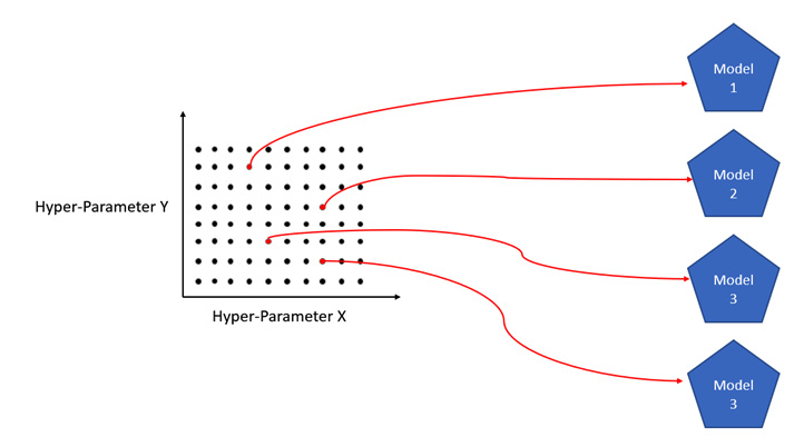
Figure 4.13 – Random grid search hyperparameter tuning

The preceding diagram is a hyperparameter space of 100 combinations of two hyperparameters, X and Y. Random grid search optimization will only choose a few at random and perform evaluations using those hyperparameter values.

The drawback of random grid search optimization is that it is a best effort approach to find the best combination of hyperparameter values with a limited number of evaluations. It may or may not find the best combination of hyperparameter values to train the optimal model, but given a large sample size, it can find the near-perfect combination to train a model with good-enough quality.

H2O library functions support random grid search optimization. It provides users with the functionality to set their own hyperparameter search grid and set a search criteria parameter to control the type and extent of the search. The search criteria can be anything, such as maximum runtime, the maximum number of models to train, or any metric. H2O will choose different hyperparameter combinations from the grid at random sequentially without repeat and will keep searching and evaluating till the search criteria are met.

H2O AutoML works slightly differently from random grid search optimization. Instead of waiting for the user to input the hyperparameter search grid, H2O has automated this part as well by already having a list of hyperparameters with all potential values for specific algorithms spaced out in the grid as default values. H2O AutoML also has provisions to include non-default values in the hyperparameter search list set by the user. H2O AutoML has predetermined values already set for algorithms; we shall explore them in the next chapter, along with understanding how different algorithms work.

Summary

In this chapter, we have come to understand the high-level architecture of H2O and what the different layers that comprise the overall architecture are. We then dived deep into the client and JVM layer of the architecture, where we understood the different components that make up the H2O software stack. Next, keeping the architecture of H2O in mind, we came to understand the flow of interactions that take place between the client and server, where we understood how exactly we command the H2O server to perform various ML activities. We also came to understand how the interactions flow down the architecture stack during model training.

Building on this knowledge, we have investigated the sequence of interactions that take place inside the H2O server during model training. We also looked into how H2O trains models using the job manager to coordinate training jobs and how H2O communicates the status of model training with the user. And, finally, we unboxed H2O AutoML and came to understand how it trains the best model automatically. We have understood the concept of hyperparameter optimization and its various approaches and how H2O automates these approaches and mitigates their drawbacks to automatically train the best model.

Now that we know the internal details of H2O AutoML and how it trains models, we are now ready to understand the various ML algorithms that H2O AutoML trains and how they manage to make predictions. In the next chapter, we shall explore these algorithms and have a better understanding of models, which will help us to justify which model would work best for a given ML problem.