3

Understanding Data Processing

A Machine Learning (ML) model is the output we get once data is fitted into an ML algorithm. It represents the underlying relationship between various features and how that relationship impacts the target variable. This relationship depends entirely on the contents of the dataset. What makes every ML model unique, despite using the same ML algorithm, is the dataset that is used to train said model. Data can be collected from various sources and can have different schemas and structures, which need not be structurally compatible among themselves but may in fact be related to each other. This relationship can be very valuable and can also potentially be the differentiator between a good and a bad model. Thus, it is important to transform this data to meet the requirements of the ML algorithm to eventually train a good model.

Data processing, data preparation, and data preprocessing are all steps in the ML pipeline that focus on best exposing the underlying relationship between the features by transforming the structure of the data. Data processing may be the most challenging step in the ML pipeline, as there are no set steps to the transformation process. Data processing depends entirely on the problem you wish to solve; however, there are some similarities among all datasets that can help us define certain processes that we can perform to optimize our ML pipeline.

In this chapter, we will learn about some of the common functionalities that are often used in data processing and how H2O has in-built operations that can help us easily perform them. We will understand some of the H2O operations that can reframe the structure of our dataframe. We will understand how to handle missing values and the importance of the imputation of values. We will then investigate how we can manipulate the various feature columns in the dataframe, as well as how to slice the dataframe for different needs. We shall also investigate what encoding is and what the different types of encoding are.

In this chapter, we are going to cover the following main topics:

• Reframing your dataframe
• Handling missing values in the dataframe
• Manipulation of feature columns of the dataframe
• Tokenization of textual data
• Encoding of data using target encoding

Technical requirements

All code examples in this chapter are run on Jupyter Notebook for an easy understanding of what each line in the code block does. You can run the whole block of code via a Python or R script executor and observe the output results, or you can follow along by installing Jupyter Notebook and observing the execution results of every line in the code blocks.

To install Jupyter Notebook, make sure you have the latest version of Python and pip installed on your system and execute the following command:

pip install jupyterlab

Once JupyterLab has successfully installed, you can start your Jupyter Notebook locally by executing the following command in your terminal:

jupyter notebook

This will open the Jupyter Notebook page on your default browser. You can then select which language you want to use and start executing the lines in the code step by step.

All code examples for this chapter can be found on GitHub at https://github.com/PacktPublishing/Practical-Automated-Machine-Learning-on-H2O/tree/main/Chapter%203.

Now, let’s begin processing our data by first creating a dataframe and reframing it so that it meets our model training requirement.

Reframing your dataframe

Data collected from various sources is often termed raw data. It is called raw in the sense that there might be a lot of unnecessary or stale data, which might not necessarily benefit our model training. The structure of the data collected also might not be consistent among all the sources. Hence, it becomes very important to first reframe the data from various sources into a consistent format.

You may have noticed that once we import the dataset into H2O, H2O converts the dataset into a .hex file, also called a dataframe. You have the option to import multiple datasets as well. Assuming you are importing multiple datasets from various sources, each with its own format and structure, then you will need a certain functionality that helps you reframe the contents of the dataset and merge them to form a single dataframe that you can feed to your ML pipeline.

H2O provides several functionalities that you can use to perform the required manipulations.

Here are some of the dataframe manipulation functionalities that help you reframe your dataframe:

• Combining columns from two dataframes
• Combining rows from two dataframes
• Merging two dataframes

Let’s see how we can combine columns from different dataframes in H2O.

Combining columns from two dataframes

One of the most common dataframe manipulation functionalities is combining different columns from different dataframes. Sometimes, the columns of one dataframe may be related to those of another. This could prove beneficial during model training. Thus, it is quite useful to have a functionality that can help us manipulate these columns and combine them together to form a single dataframe for model training.

H2O has a function called cbind() that combines the columns from one dataset into another.

Let’s try this function out in our Jupyter Notebook using Python. Execute the following steps in sequence:

1. Import the h2o library:

   import h2o

2. Import the numpy library; we will use this to create a sample dataframe for our study:

   import numpy as np

3. Initialize the h2o server:

   h2o.init()

4. Now, let’s create a dataframe called important_dataframe_1; this is a dataframe whose columns are important. To ensure that you generate the same values in the dataset as in this example, set the random seed value for numpy to 123. We will set the number of rows to 15 and the number of columns to 5. You can name the columns anything you like:

   np.random.seed(123)

   important_dataframe_1 = h2o.H2OFrame.from_python(np.random.randn(15,5).tolist(), column_names=list([" important_column_1" , " important_column_2" , " important_column_3" , " important_column_4" , " important_column_5" ]))

5. Let’s check out the content of the dataset by executing the following code:

   important_dataframe_1.describe

The following screenshot shows you the contents of the dataset:

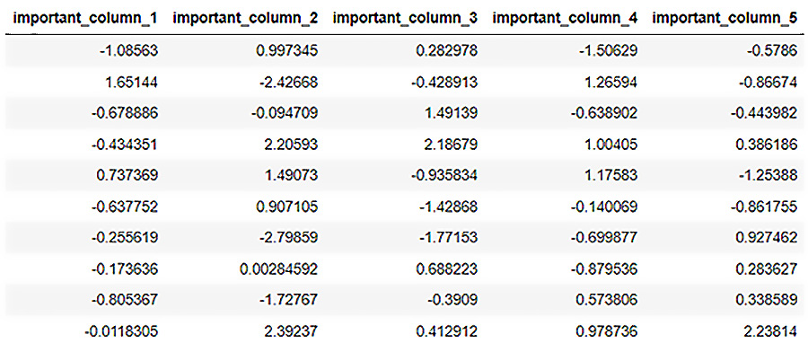
Figure 3.1 – important_dataframe_1 data content

6. Let’s create another dataframe called important_dataframe_2, as before but with different column names, but an equal number of rows and only 2 columns:

   important_dataframe_2 = h2o.H2OFrame.from_python(np.random.randn(15,2).tolist(), column_names=list([" important_column_6" , " important_column_7" ]))

7. Let’s check out the content of this dataframe as well:

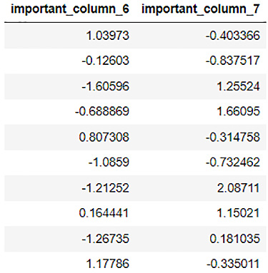
Figure 3.2 – important_dataframe_2 data content

8. Now, let’s combine the columns of both the dataframes and store them in another variable called final_dataframe, using the cbind() function:

   final_dataframe = important_dataframe_1.cbind(important_dataframe_2)

9. Let’s now observe final_dataframe:

   final_dataframe.describe

You should see the contents of final_dataframe as follows:

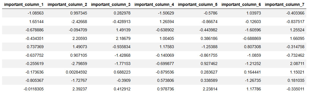
Figure 3.3 – final_dataframe data content after cbind()

Here, you will notice that we have successfully combined the columns from important_dataframe_2 with the columns of important_dataframe_1.

This is how you can use the cbind() function to combine the columns of two different datasets into a single dataframe. The only thing to bear in mind while using the cbind() function is that it is necessary to ensure that both the datasets to be combined have the same number of rows. Also, if you have dataframes with the same column name, then H2O will append a 0 in front of the column from dataframe.

Now that we know how to combine the columns of different dataframes, let’s see how we can combine the column values of multiple dataframes with the same column structure.

Combining rows from two dataframes

The majority of big corporations often handle tremendous amounts of data. This data is often partitioned into multiple chunks to make storing and reading it faster and more efficient. However, during model training, we will often need to access all these partitioned datasets. These datasets have the same structure but the data contents are distributed. In other words, the dataframes have the same columns; however, the data values or rows are split among them. We will often need a function that combines all these dataframes together so that we have all the data values available for model training.

H2O has a function called rbind() that combines the rows from one dataset into another.

Let’s try this function out in the following example:

1. Import the h2o library:

   import h2o

2. Import the numpy library; we will use this to create a random dataframe for our study:

   import numpy as np

3. Initialize the h2o server:

   h2o.init()

4. Now, let’s create a random dataframe called important_dataframe_1. To ensure that you generate the same values in the dataset as in this example, set the random seed value for numpy to 123. We will set the number of rows to 15 and the number of columns to 5. You can name the columns anything you like:

   np.random.seed(123)

   important_dataframe_1 = h2o.H2OFrame.from_python(np.random.randn(15,5).tolist(), column_names=list([" important_column_1" , " important_column_2" ," important_column_3" ," important_column_4" ," important_column_5" ]))

5. Let’s check out the number of rows of the dataframe, which should be 15:

   important_dataframe_1.nrows

6. Let’s create another dataframe called important_dataframe_2, as with the previous one, with the same column names and any number of rows. In the example, I have used 10 rows:

   important_dataframe_2 = h2o.H2OFrame.from_python(np.random.randn(10,5).tolist(), column_names=list([" important_column_1" , " important_column_2" ," important_column_3" ," important_column_4" ," important_column_5" ]))

7. Let’s check out the number of rows for important_dataframe_2, which should be 10:

   important_dataframe_2.nrows

8. Now, let’s combine the rows of both the dataframes and store them in another variable called final_dataframe, using the rbind() function:

   final_dataframe = important_dataframe_1.rbind(important_dataframe_2)

9. Let’s now observe final_dataframe:

   final_dataframe.describe

You should see the contents of final_dataframe as follows:

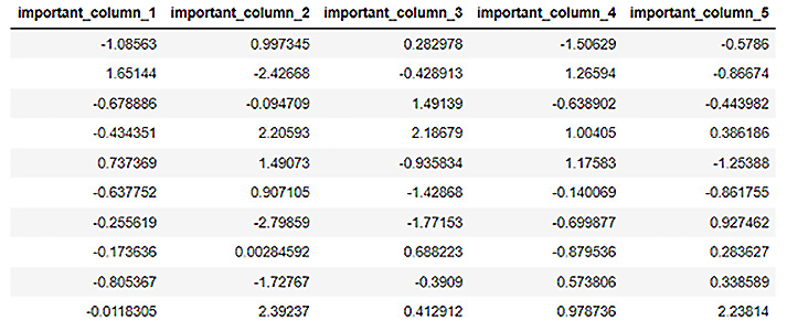
Figure 3.4 – final_dataframe data contents after rbind()

10. Let’s check out the number of rows in final_dataframe:

    final_dataframe.nrows

The output of the last operation should show you the value of the number of rows in the final dataset. You will see that the value is 25 and the contents of the dataframe are the combined row values of both the previous datasets.

Now that we have understood how to combine the rows of two dataframes in H2O using the rbind() function, let’s see how we can fully combine two datasets.

Merging two dataframes

You can directly merge two dataframes, combining their rows and columns into a single dataframe. H2O provides a merge() function that combines two datasets that share a common column or common columns. During merging, columns that the two datasets have in common are used as the merge key. If they only have one column in common, then that column forms the singular primary key for the merge. If there are multiple common columns, then H2O will form a complex key of all these columns based on their data values and use that as the merge key. If there are multiple common columns between the two datasets and you only wish to merge a specific subset of them, then you will need to rename the other common columns to remove the corresponding commonality.

Let’s try this function out in the following example in Python:

1. Import the h2o library:

   import h2o

2. Import the numpy library; we will use this to create a random dataframe for our study:

   import numpy as np

3. Initialize the h2o server:

   h2o.init()

4. Now, let’s create a dataframe called dataframe_1. The dataframe has 3 columns: words, numerical_representation, and letters. Now, let’s fill in the data content as follows:

   dataframe_1 = h2o.H2OFrame.from_python({'words':['Hello', 'World', 'Welcome', 'To', 'Machine', 'Learning'], 'numerical_representation': [0,1,2,3,4,5],'letters':['a','b','c','d']})

5. Let’s check out the content of the dataset:

   dataframe_1.describe

6. You will notice the contents of the dataset as follows:
   

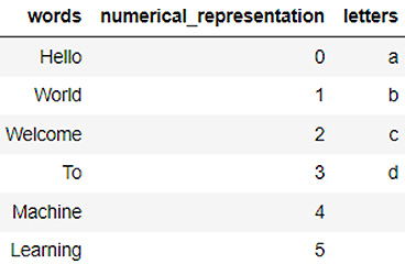
Figure 3.5 – dataframe_1 data content

7. Let’s create another dataframe called dataframe_2. This dataframe also contains 3 columns: the numerical_representation column, the letters column (both of which it has in common with dataframe_1), and an uncommon column. Let’s call it other_words:

   dataframe_2 = h2o.H2OFrame.from_python({'other_words':['How', 'Are', 'You', 'Doing', 'Today', 'My', 'Friend', 'Learning', 'H2O', 'Artificial', 'Intelligence'], 'numerical_representation': [0,1,2,3,4,5,6,7,8,9],'letters':['a','b','c','d','e']})

8. Let’s check out the content of this dataframe as well:

   dataframe_2.head(11)

On executing the code, you should see the following output in your notebook:

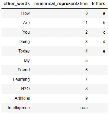
Figure 3.6 – dataframe_2 data contents

9. Now, let’s merge dataframe_1 into dataframe_2, using the merge() operation:

   final_dataframe = dataframe_2.merge(dataframe_1)

10. Let’s now observe final_dataframe:

    final_dataframe.describe

11. You should see the contents of final_dataframe as follows:

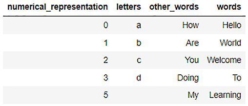
Figure 3.7 – final_dataframe contents after merge()

You will notice that H2O used the combination of the numerical_representation column and the letters column as the merging key. This is why we have values ranging from 1 to 5 in the numerical_representation column with the appropriate values in the other columns.

Now, you may be wondering why there is no row for 4. That is because while merging, we have two common columns: numerical_representation and letters. So, H2O used a complex merging key that uses both these columns: (0, a), (1, b), (2, c), and so on.

Now the next question you might have is What about the row with the value 5? It has no value in the letters column. That is because even an empty value is treated as a unique value in ML. Thus, during merging, the complex key that was generated treated (5, ) as a valid merge key.

H2O drops all the remaining values since dataframe_1 does not have any more numerical representation values.

12. You can enforce H2O to not drop any of the values from the merge key column by setting the all_x parameter to True as follows:

    final_dataframe = dataframe_2.merge(dataframe_1, all_x = True)

13. Now, let’s observe the contents of final_dataframe by using its describe attribute:

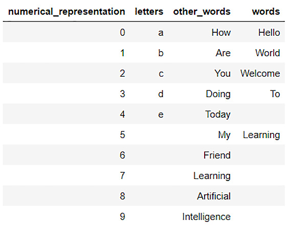
Figure 3.8 – final_dataframe data content after enforcing merge()

You will notice that we now have all the values from both dataframes merged into a single dataframe. We have all the numerical representations from 0 to 9 and all letters from a to e from dataframe_2 that were missing in the previous step, along with the correct values from the other_words column and the words column.

To recap, we learned how to combine dataframe columns and rows. We also learned how to combine entire dataframes together using the merge() function. However, we noticed that if we enforced the merging of dataframes despite them not having common data values in their key columns, we ended up with missing values in the dataframe.

Now, let’s look at the different methods we can use to handle missing values using H2O.

Handling missing values in the dataframe

Missing values in datasets are the most common issue in the real world. It is often expected to have at least a few instances of missing data in huge chunks of datasets collected from various sources. Data can be missing for several reasons, which can range from anything from data not being generated at the source all the way to downtimes in data collectors. Handling missing data is very important for model training, as many ML algorithms don’t support missing data. Those that do may end up giving more importance to looking for patterns in the missing data, rather than the actual data that is present, which distracts the machine from learning.

Missing data is often referred to as Not Available (NA) or nan. Before we can send a dataframe for model training, we need to handle these types of values first. You can either drop the entire row that contains any missing values or you can fill them with any default value either default or common for that data column. How you handle missing values depends entirely on which data is missing and how important it is for the overall model training.

H2O provides some functionalities that you can use to handle missing values in a dataframe. These are some of them:

• The fillna() function
• Replacing values in a frame
• Imputation

Next, let’s see how we can fill missing values in a dataframe using H2O.

Filling NA values

fillna() is a function in H2O that you can use to fill missing data values in a sequential manner. This is especially handy if you have certain data values in a column that are sequential in nature, for example, time series or any metric that increases or decreases sequentially and can be sorted. The smaller the difference between the values in the sequence, the more applicable this function becomes.

The fillna() function has the following parameters:

• method: This can either be forward or backward. It indicates the direction in which H2O should start filling the NA values in the dataframe.
• axis: 0 for column-wise fill or 1 for row-wise fill.
• maxlen: The maximum number of consecutive NAs to fill.

Let’s see an example in Python of how we can use this function to fill missing values:

1. Import the h2o library:

   import h2o

2. Import the numpy library; we will use this to create a random dataframe for our study:

   import numpy as np

3. Initialize the h2o server:

   h2o.init()

4. Create a random dataframe with 1000 rows, 3 columns, and some NA values:

   dataframe = h2o.create_frame(rows=1000, cols=3, integer_fraction=1.0, integer_range=100, missing_fraction=0.2, seed=123)

5. Let’s observe the contents of this dataframe. Execute the following code and you will see certain missing values in the dataframe:

   dataframe.describe

You should see the contents of the dataframe as follows:

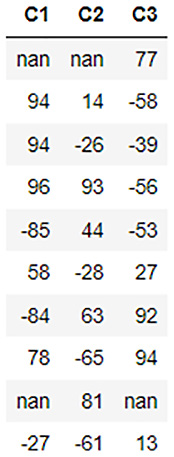
Figure 3.9 – Dataframe contents

6. Let’s now use the fillna() function to forward fill the NA values. Execute the following code:

   filled_dataframe = dataframe.fillna(method=" forward" , axis=0, maxlen=1)

7. Let’s observe the filled contents of the dataframe. Execute the following code:

   filled_dataframe.describe

8. You should see the contents of the dataframe as follows:

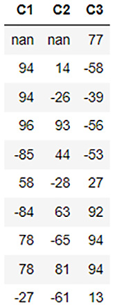
Figure 3.10 – filled_dataframe contents

The fillna() function has filled most of the NA values in the dataframe sequentially.

However, you will notice that we still have some nan values in the first row of the dataframe. This is because we filled the dataframe missing values row-wise in the forward direction. When filling NA values, H2O will record the last value in a row for a specific column and copy it if the value in the subsequent row is NA. Since this is the very first column, H2O does not have any previous value in the record to fill it, thus it skips over it.

Now that we understand how we can sequentially fill data in a dataframe using the fillna() function in H2O, let’s see how we can replace certain values in the dataframe.

Replacing values in a frame

Another common functionality often needed for data processing is replacing certain values in the dataframe. There can be plenty of reasons why you might want to do this. This is especially common for numerical data where some of the most common transformations include rounding off values, normalizing numerical ranges, or just correcting a data value. In this section, we will explore some of the functions that we can use in H2O to replace values in the dataframe.

Let’s first create a dataframe that we can use to test out such functions. Execute the following code so that we have a dataframe ready for manipulation:

import h2o
h2o.init()
dataframe = h2o.create_frame(rows=10, cols=3, real_range=100, integer_fraction=1, missing_fraction=0.1, seed=5)
dataframe.describe

The dataframe should look as follows:

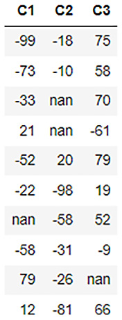
Figure 3.11 – Dataframe data contents

So, we have a dataframe with three columns: C1, C2, and C3. Each column has a few negative numbers and some nan values. Let’s see how we can play around with this dataframe.

Let’s start with something simple. Let’s update the value of a single data value, also called a datum, in the dataframe. Let’s update the fourth row of the C2 column to 99. You can update the value of a single data value based on its position in the dataframe as follows:

dataframe[3,1] = 99

Note that the columns and rows in the dataframe all start with 0. Hence, we set the value in the dataframe with the row number of 3 and the column number of 1 as 99. You should see the results in the dataframe by executing dataframe.describe as follows:

dataframe.describe

The dataframe should look as follows:

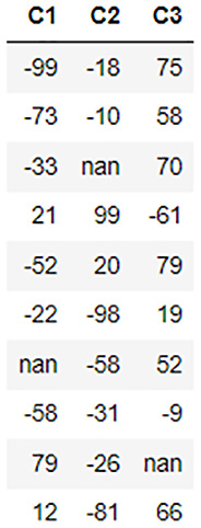
Figure 3.12 – Dataframe contents after the datum update

As you can see in the dataframe, we replaced the nan value that was previously in the third row of the C2 column with 99.

This is a manipulation of just one data value. Let’s see how we can replace the values of an entire column. Let’s increase the data values in the C3 column to three times their original value. You can do so by executing the following code:

dataframe[2] = 3*dataframe[2]

You should see the results in the dataframe by executing dataframe.describe as follows:

dataframe.describe

The dataframe should look as follows:

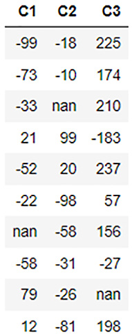
Figure 3.13 – Dataframe contents after column value updates

We can see in the output that the values in the C3 column have now been increased to three times the original values in the column.

All these replacements we performed till now are straightforward. Let’s try some conditional updates on the dataframe. Let’s round off all the negative numbers in the dataframe to 0. So, the condition is that we only update the negative numbers to 0 and don’t change any of the positive numbers. You can do conditional updates as follows:

dataframe[dataframe['C1'] < 0, " C1" ] = 0
dataframe[dataframe['C2'] < 0, " C2" ] = 0
dataframe[dataframe['C2'] < 0, " C3" ] = 0

You should see the results in the dataframe by executing dataframe.describe as follows:

dataframe.describe

The dataframe should look as follows:

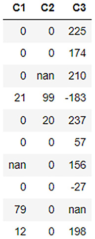
Figure 3.14 – Dataframe contents after conditional updates

As you can see in the dataframe, all the negative values have been rounded up/replaced by 0.

Now, what if instead of rounding the negative numbers up to 0 we wished to just inverse the negative numbers? We could do so by combining the conditional updates with arithmetic updates. Refer to the following example:

dataframe[" C1" ] = (dataframe[" C1" ] < 0).ifelse(-1*dataframe[" C1" ], dataframe[" C1" ])
dataframe[" C2" ] = (dataframe[" C2" ] < 0).ifelse(-1*dataframe[" C2" ], dataframe[" C2" ])
dataframe[" C3" ] = (dataframe[" C3" ] < 0).ifelse(-1*dataframe[" C3" ], dataframe[" C3" ])

Now, let’s try to see whether we can replace the remaining nan values with something valid. We already read about the fillna() function, but what if the nan values are nothing but some missing values that don’t exactly fall into any incremental or decremental pattern, and we just want to set it to 0? Let’s do that now. Run the following code:

dataframe[dataframe[" C1" ].isna(), " C1" ] = 0
dataframe[dataframe[" C2" ].isna(), " C2" ] = 0
dataframe[dataframe[" C3" ].isna(), " C3" ] = 0

You should see the results in the dataframe by executing dataframe.describe as follows:

dataframe.describe

The dataframe should look as follows:

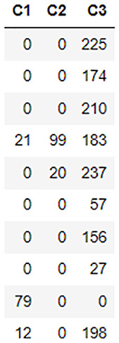
Figure 3.15 – Dataframe contents after replacing nan values with 0

The isna() function is a function that checks whether the value in the datum is nan or not and returns either True or False. We use this condition to replace the values in the dataframe.

Tip

There are plenty of ways to manipulate and replace the values in a dataframe and H2O provides plenty of functionality to make implementation easy. Feel free to explore and experiment more with manipulating the values in the dataframe. You can find more details here: https://docs.h2o.ai/h2o/latest-stable/h2o-py/docs/frame.html.

Now that we have learned various methods to replace values in the dataframe, let’s look into a more advanced approach to doing so that data scientists and engineers often take.

Imputation

Previously, we have seen how we can replace nan values in the dataset using fillna(), which sequentially replaces the nan data in the dataframe. The fillna() function fills data in a sequential manner; however, data need not always be sequential in nature. For example, consider a dataset of people buying gaming laptops. The dataset will mostly contain data about people in the age demographic of 13-28, with a few outliers. In such a scenario, if there are any nan values in the age column of the dataframe, then we cannot use the fillna() function to fill the nan values, as any nan value after any outlier value will introduce a bias in the dataframe. We need to replace the nan value with a value that is common among the standard distribution of the age group for that product, something that is between 13 and 28, rather than say 59, which is less likely.

Imputation is the process of replacing certain values in the dataframe with an appropriate substitute that does not introduce any bias or outliers that may impact model training. The method or formulas used to calculate the substitute value are termed the imputation strategy. Imputation is one of the most important methods of data processing, which handles missing and nan values and tries to replace them with a value that will potentially introduce the least bias into the model training process.

H2O has a function called impute() that specifically provides this functionality. It has the following parameters:

• column: This parameter accepts the column number that sets the columns to impute(). The value 1 imputes the entire dataframe.
• method: This parameter sets which method of imputation to use. The methods can be either mean, median, or mode.
• combine_method: This parameter dictates how to combine the quantiles for even samples when the imputation method chosen is median. The combination methods are either interpolate, average, low, or high.
• group_by_frame: This parameter imputes the values of the selected precomputed grouped frame.
• by: This parameter groups the imputation results by the selected columns.
• values: This parameter accepts a list of values that are imputed per column. Having the None value in the list skips the column.

Let’s see an example in Python of how we can use this function to fill missing values.

For this, we shall use the high school student sprint dataset. The high school student sprint dataset is a dataset that consists of recordings of the age of high school students, their weight, maximum recorded speed, and their performance in a 100-meter sprint. The dataset is used to predict how the age, weight, and sprint speed affect the performance of students in a 100-meter sprint race.

The dataset looks as follows:

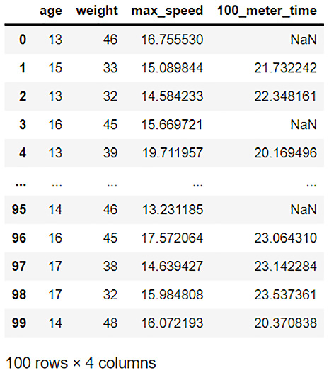
Figure 3.16 – A high school student sprint dataset

The features of the dataset are as follows:

• age: Age of the student
• weight: Weight of the student in kilograms
• max_speed: The maximum sprint speed of the student in kilometers per hour
• 100_meter_time: The time taken by the student to finish a 100-meter sprint in seconds

As you can see, there are plenty of missing values in the 100_meter_time column.

We cannot simply use the fillna() function, as that will introduce bias into the data if the missing values happen to be right after the fastest or slowest time. We can’t simply replace the values with a constant number either.

What would actually make sense is to replace these missing values with whatever is normal for an average teenager doing a 100-meter dash. We already have values for the majority of students, so we can use their results to calculate a general average 100-meter sprint time and use that as a baseline to replace all the missing values without introducing any bias.

This is exactly what imputation is used for. Let’s use the imputation function to fill in these missing values:

1. Import the h20 module and start the h20 server:

   import h2o

   h2o.init()

2. We then import the high school student sprint dataset by using h2o.import_file():

   dataframe = h2o.import_file(" Dataset/high_school_student_sprint.csv" )

3. Using the impute() function, let’s impute the missing values in the 100_meter_time column by mean and display the data:

   dataframe.impute(" 100_meter_time" , method = " mean" )

   dataframe.describe

You will see the output of the imputed dataframe as follows:

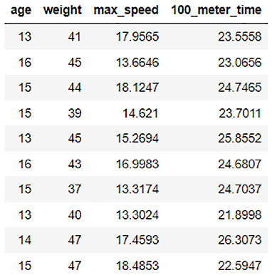
Figure 3.17 – 100_meter_time column imputed by its mean

4. H2O calculated the mean value of all the values in the 100_meter_time column as 23.5558 and replaced the missing values with it.

Similarly, instead of mean, you can use median values as well. However, note that if a column has categorical values, then the method must be mode. The decision is up to you to make, depending on the dataset that is most useful when replacing the missing values:

dataframe.impute(" 100_meter_time" , method = " median" )

dataframe.impute(" 100_meter_time" , method = " mode" )

5. Let’s increase the complexity a bit. What if the average 100-meter sprint time is not truly comparable between all students? What if the performances are more comparable age-wise? For example, students of age 16 are faster than the ones who are 13 since they are more physically developed. In that case, it won’t make sense considering a 13-year-old’s sprint time when imputing the missing value of a 16-year-old. This is where we can use the group parameter of the impute() function:

   dataframe = h2o.import_file(" Dataset/high_school_student_sprint.csv" )

   dataframe.impute(" 100_meter_time" , method = " mean" , by=[" age" ])

   dataframe.describe

You will see the output as follows:

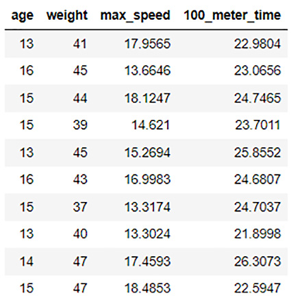
Figure 3.18 – 100_meter_sprint imputed by its mean and grouped by age

You will notice that now H2O has calculated the mean values by age and replaced the respective missing values for that age in the 100_meter_time column. Observe the first row in the dataset. The row was of students aged 13 and had missing values in its 100_meter_time column. It was replaced with the mean value of all the 100_meter_time values for other 13-year-olds. Similar steps were followed for other age groups. This is how you can use the group by parameter in the impute() function to flexibly impute the correct values.

The impute() function is extremely powerful to impute the correct values in a dataframe. The additional parameters for grouping via columns as well as frames make it very flexible for use in handling all sorts of missing values.

Feel free to use and explore all these functions on different datasets. At the end of the day, all these functions are just tools used by data scientists and engineers to improve the quality of the data; the real skill is understanding when and how to use these tools to get the most out of your data, and that requires experimentation and practice.

Now that we have learned about the different ways in which we can handle missing data, let’s move on to the next part of data processing, which is how to manipulate the feature columns of the dataframe.

Manipulating feature columns of the dataframe

The majority of the time, your data processing activities will mostly involve manipulating the columns of the dataframes. Most importantly, the type of values in the column and the ordering of the values in the column will play a major role in model training.

H2O provides some functionalities that help you do so. The following are some of the functionalities that help you handle missing values in your dataframe:

• Sorting of columns
• Changing the type of the column

Let’s first understand how we can sort a column using H2O.

Sorting columns

Ideally, you want the data in a dataframe to be shuffled before passing it off to model training. However, there may be certain scenarios where you might want to re-order the dataframe based on the values in a column.

H2O has a functionality called sort() to sort dataframes based on the values in a column. It has the following parameters:

• by: The column to sort by. You can pass multiple column names as a list as well.
• ascending: A boolean array that denotes the direction in which H2O should sort the columns. If True, H2O will sort the column in ascending order. If False, then H2O will sort it in descending order. If neither of the flags is passed, then H2O defaults to sorting in ascending order.

The way H2O will sort the dataframe depends on whether one column name is passed to the sort() function or multiple column names. If only a single column name is passed, then H2O will return a frame that is sorted by that column.

However, if multiple columns are passed, then H2O will return a dataframe that is sorted as follows:

• H2O will first sort the dataframe on the first column that is passed in the parameter.
• H2O will then sort the dataframe on the next column passed in the parameter, but only those rows will be sorted that have the same values as in the first sorted column. If there are no duplicate values in the previous columns, then no sorting will be done on subsequent columns.

Let’s see an example in Python of how we can use this function to sort columns:

1. Import the h2o library and initialize it:

   import h2o

   h2o.init()

2. Create a dataframe by executing the following code and observe the dataset:

   dataframe = h2o.H2OFrame.from_python({'C1': [3,3,3,0,12,13,1,8,8,14,15,2,3,8,8],'C2':[1,5,3,6,8,6,8,7,6,5,1,2,3,6,6],'C3':[15,14,13,12,11,10,9,8,7,6,5,4,3,2,1]})

   dataframe.describe

The contents of the dataset should be as follows:

Figure 3.19 – dataframe_1 data contents

3. So, at the moment, the values in columns C1, C2, and C3 are all random in nature. Let’s use the sort() function to sort the dataframe by column C1. You can do so by either passing 0 into the by parameter, indicating the first column of the dataframe, or by passing [‘C1’], which is a list containing column names to sequentially sort the dataset:

   sorted_dataframe_1 = dataframe.sort(0)

   sorted_dataframe_1.describe

You should get an output of the code as follows:

Figure 3.20 – dataframe_1 sorted by the C1 column

You will see that the dataframe is now sorted in ascending order by the C1 column.

4. Let’s see what we shall get if we pass multiple columns in the by parameter to sort on multiple columns. Run the following code line:

   sorted_dataframe_2 = dataframe.sort(['C1','C2']) sorted_dataframe_2.describe

You should get an output as follows:

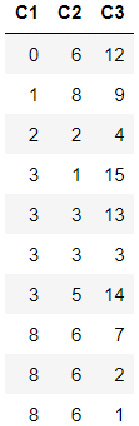
Figure 3.21 – dataframe_1 sorted by columns C1 and C2

As you can see, H2O first sorted the columns by the C1 column. Then, it sorted the rows by the C2 column for those rows that had the same value in the C1 column. H2O will sequentially sort the dataframe column-wise for all the columns you pass in the sort function.

5. You can also reverse the sorting order by passing False in the ascending parameter. Let’s test this out by running the following code line:

   sorted_dataframe_3 = dataframe.sort(by=['C1','C2'], ascending=[True,False])

   sorted_dataframe_3.describe

You should see an output as follows:

Figure 3.22 – dataframe_1 sorted by the C1 column in ascending order and the C2 column in descending order

In this case, H2O first sorted the columns by the C1 column. Then, it sorted the rows by the C2 column for those rows that had the same value in the C1 column. However, this time it sorted the values in descending order.

Now that you’ve learned how to sort the dataframe by a single column as well as by multiple columns, let’s move on to another column manipulation function that changes the type of the column.

Changing column types

As we saw in Chapter 2, Working with H2O Flow (H2O’s Web UI), we changed the type of the Heart Disease column to enum from numerical. The reason we did this is that the type of column plays a major role in model training. During model training, the type of column decides whether the ML problem is a classification problem or a regression problem. Despite the fact that the data in both cases is numerical in nature, how a ML algorithm will treat the column depends entirely on its type. Thus, it becomes very important to correct the types of columns that might not be correctly set during the initial stages of data collection.

H2O has several functions that not only help you change the type of the columns but also run initial checks on the column types.

Some of the functions are as follows:

• .isnumeric(): Checks whether the column in the dataframe is of the numeric type. Returns True or False accordingly
• .asnumeric(): Creates a new frame with all the values converted to numeric for the specified column
• .isfactor(): Checks whether the column in the dataframe is of categorical type. Returns True or False accordingly
• .asfactor(): Creates a new frame with all the values converted to the categorical type for the specified column
• .isstring(): Checks whether the column in the dataframe is of the string type. Returns True or False accordingly
• .ascharacter(): Creates a new frame with all the values converted to the string type for the specified column

Let’s see an example in Python of how we can use these functions to change the column types:

1. Import the h2o library and initialize H2O:

   import h2o

   h2o.init()

2. Create a dataframe by executing the following code line and observe the dataset:

   dataframe = h2o.H2OFrame.from_python({'C1': [3,3,3,0,12,13,1,8,8,14,15,2,3,8,8],'C2':[1,5,3,6,8,6,8,7,6,5,1,2,3,6,6],'C3':[15,14,13,12,11,10,9,8,7,6,5,4,3,2,1]})

   dataframe.describe

The contents of the dataset should be as follows:

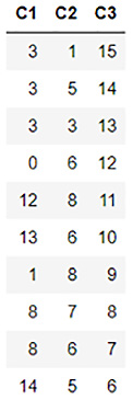
Figure 3.23 – Dataframe data contents

3. Let’s confirm whether the C1 column is a numerical column by using the isnumeric() function as follows:

   dataframe['C1'].isnumeric()

You should get an output of True.

4. Let’s see what we get if we check whether the C1 column is a categorical column using the asfactor() function as follows:

   dataframe['C1'].isfactor()

You should get an output of False.

5. Now let’s convert the C1 column to a categorical column using the asfactor() function and then check whether isfactor() returns True:

   dataframe['C1'] = dataframe['C1'].asfactor()

   dataframe['C1'].isfactor()

You should now get an output of True.

6. You can convert the C1 column back into a numerical column by using the asnumeric() function:

   dataframe['C1'] = dataframe['C1'].asnumeric()

   dataframe['C1'].isnumeric()

You should now get an output of True.

Now that you have learned how to sort the columns of a dataframe and change column types, let’s move on to another important topic in data processing, which is tokenization and encoding.

Tokenization of textual data

Not all Machine Learning Algorithms (MLAs) are focused on mathematical problem-solving. Natural Language Processing (NLP) is a branch of ML that specializes in analyzing meaning out of textual data, though it will try to derive meaning and understand the contents of a document or any text for that matter. Training an NLP model can be very tricky, as every language has its own grammatical rules and the interpretation of certain words depends heavily on context. Nevertheless, an NLP algorithm often tries its best to train a model that can predict the meaning and sentiments of a textual document.

The way to train an NLP algorithm is to first break down the chunk of textual data into smaller units called tokens. Tokens can be words, characters, or even letters. It depends on what the requirements of the MLA are and how it uses these tokens to train a model.

H2O has a function called tokenize() that helps break down string data in a dataframe into tokens and creates a separate column containing all the tokens for further processing.

It has the following parameter: split: We pass a regular expression in this parameter that will be used by the function to split the text data into tokens.

Let’s see an example of how we can use this function to tokenize string data in a dataframe:

1. Import the h2o library and initialize it:

   import h2o

   h2o.init()

2. Create a dataframe by executing the following code line and observe the dataset:

   dataframe1 = h2o.H2OFrame.from_python({'C1':['Today we learn AI', 'Tomorrow AI learns us', 'Today and Tomorrow are same', 'Us and AI are same']})

   dataframe1 = dataframe1.ascharacter()

   dataframe1.describe

The dataset should look as follows:

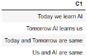
Figure 3.24 – Dataframe data contents

This type of textual data is usually collected in systems that generate a lot of log text or conversational data. To solve such NLP tasks, we need to break down the sentences into individual tokens so that we can eventually build the context and meaning of these texts that will help the ML algorithm to make semantic predictions. However, before diving into the complexities of NLP, data scientists and engineers will process this data by tokenizing it first.

3. Let’s tokenize our dataframe using this function to split the text with blank spaces and observe the tokenized column:

   tokenized_dataframe = dataframe1.tokenize("  " )

   tokenized_dataframe

You should see the dataframe as follows:

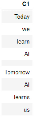
Figure 3.25 – Tokenized dataframe data contents

You will notice that the tokenize() function splits the text data into tokens and appends the tokens as rows into a single column. You will also notice that all tokenized sentences are separated by empty rows. You can cross-check this by comparing the number of words in all the sentences in the dataframe, plus the empty spaces between the sentences against the number of rows in the tokenized dataset, using nrows.

These are some of the most used data processing methods that are used to process your data before you feed it to your ML pipeline for training. There are still plenty of methods and techniques that you can use to further clean and polish your dataframes. So much so that you could dedicate an entire book to discussing them. Data processing happens to be the most difficult part of the entire ML life cycle. The quality of the data used for training depends on the context of the problem statement. It also depends on the creativity and ingenuity of the data scientists and engineers in processing that data. The end goal of data processing is to extract as much information as we can from the dataset and remove noise and bias from the data to allow for a more efficient analysis of data during training.

Encoding data using target encoding

As we know, machines are only capable of understanding numbers. However, plenty of real-world ML problems revolve around objects and information that are not necessarily numerical in nature. Things such as states, names, and classes, in general, are represented as categories rather than numbers. This kind of data is called categorical data. Categorical data will often play a big part in analysis and prediction. Hence, there is a need to convert these categorical values to a numerical format so that machines can understand them. The conversion should also be in such a way that we do not lose the inherent meaning of those categories, nor do we introduce new information into the data, such as the incremental nature of numbers, for example.

This is where encoding is used. Encoding is a process where categorical values are transformed, in other words, encoded, into numerical values. There are plenty of encoding methods that can perform this transformation. One of the most commonly used ones is target encoding.

Target encoding is an encoding process that transforms categorical values into numerical values by calculating the average probability of the target variable occurring for a given category. H2O also has methods that help users implement target encoding on their data.

To better understand this method, consider the following sample Mythical creatures dataset:

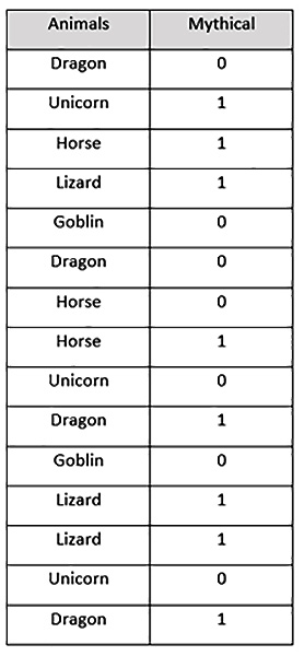
Figure 3.26 – Our mythical creatures dataset

This dataset has the following content:

• Animals: This column contains categorical values of the names of animals.
• Mythical: This column contains the 0 binary value and the 1 binary value. 1 indicates that the creature is mythical, while 0 indicates that the creature is not mythical.

Now, let’s encode the Animals categorical column using target encoding. Target encoding will perform the following steps:

1. Group the categorical values and record the number of times the target value, Mythical, was 1 and when it was 0 for a given category as follows:

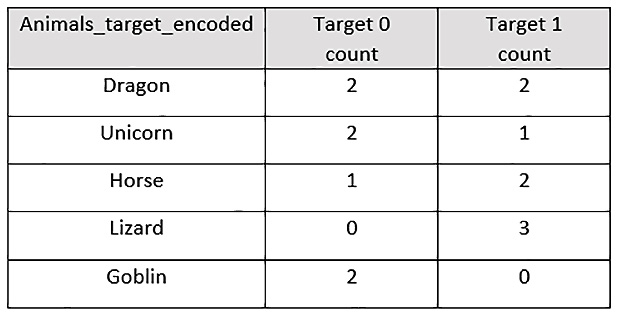
Figure 3.27 – The mythical creatures dataset with a target count

2. Calculate the probability that the 1 target value will occur, as compared to the 0 target value within each specific group. This would look as follows:

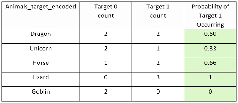
Figure 3.28 – The mythical creatures dataset with a Probability of Target 1 Occurring column

3. Drop the Animals column and use the Probability of Target 1 Occurring column as the encoded representation of the Animals column. The new encoded dataset will look as follows:

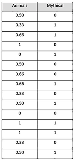
Figure 3.29 – A target-encoded mythical creatures dataset

In the encoded dataset, the Animals feature is encoded using target encoding and we have a dataset that is entirely numerical in nature. This dataset will be easy for an ML algorithm to interpret and learn from, providing high-quality models.

Let us now see how we can perform target encoding using H2O. The dataset we will use for this example is the Automobile price prediction dataset. You can find the details of this dataset at https://archive.ics.uci.edu/ml/datasets/Automobile (Dua, D. and Graff, C. (2019). UCI Machine Learning Repository [http://archive.ics.uci.edu/ml]. Irvine, CA: University of California, School of Information and Computer Science).

The dataset is fairly straightforward. It contains various details about cars, such as the make of the car, engine size, fuel system, compression ratio, and price. The aim of the ML algorithm is to predict the price of a car based on these features.

For our experiment, we shall encode the categorical columns make, fuel type, and body style using target encoding where the price column is the target.

Let’s perform target encoding by following this example:

1. Import h2o and H2O’s target encoder library, H2OTargetEncoderEstimator, and initialize your H2O server. Execute the following code:

   import h2o

   from h2o.estimators import H2OTargetEncoderEstimator

   h2o.init()

2. Import the Automobile price prediction dataset and print the contents of the dataset. Execute the following code:

   automobile_dataframe = h2o.import_file(" DatasetAutomobile_data.csv" )

   automobile_dataframe

Let’s observe the contents of the dataframe; it should look as follows:

Figure 3.30 – An automobile price prediction dataframe

As you can see in the preceding figure, the dataframe consists of a large number of columns containing the details of cars. For the sake of understanding target encoding, let’s filter out the columns that we want to experiment with while dropping the rest. Since we plan on encoding the make column, the fuel-type column, and the body-style column, let’s use only those columns along with the price response column. Execute the following code:

automobile_dataframe = automobile_dataframe[:,[" make" , " fuel-type" , " body-style" , " price" ]]

automobile_dataframe

The filtered dataframe will look as follows:

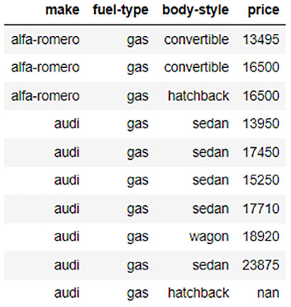
Figure 3.31 – The automobile price prediction dataframe with filtered columns

3. Let’s now split this dataframe into training and testing dataframes. Execute the following code:

   automobile_dataframe_for_training, automobile_dataframe_for_test = automobile_dataframe.split_frame(ratios = [.8], seed = 123)

4. Let’s now train our target encoder model using H2OTargetEncoderEstimator. Execute the following code:

   automobile_te = H2OTargetEncoderEstimator()

   automobile_te.train(x= [" make" , " fuel-type" , " body-style" ], y=" price" , training_frame=automobile_dataframe_for_training)

Once the target encoder has finished its training, you will see the following output:

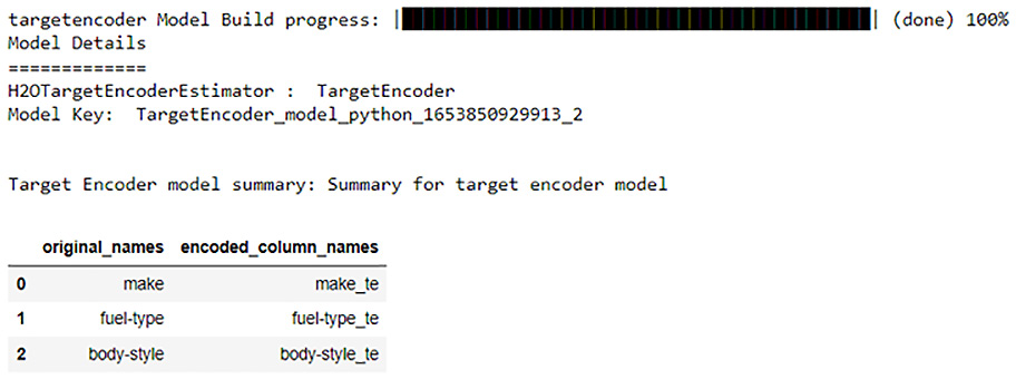
Figure 3.32 – The result of target encoder training

From the preceding screenshot, you can see that the H2O target encoder will generate the target-encoded values for the make column, the fuel-type column, and the body-style column and store them in different columns named make_te, fuel-type_te, and body-style_te, respectively. These new columns will contain the encoded values.

5. Let’s now use this trained target encoder to encode the training dataset and print the encoded dataframe:

   te_automobile_dataframe_for_training = automobile_te.transform(frame=automobile_dataframe_for_training, as_training=True)

   te_automobile_dataframe_for_training

The encoded training frame should look as follows:

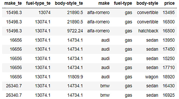
Figure 3.33 – An encoded automobile price prediction training dataframe

As you can see from the figure, our training frame now has three additional columns, make_te, fuel-type_te, and body-style_te, with numerical values. These are the target-encoded columns for the make column, the fuel-type column, and the body-style column.

6. Similarly, let’s now use the trained target encoder to encode the test dataframe and print the encoded dataframe. Execute the following code:

   te_automobile_dataframe_for_test = automobile_te.transform(frame=automobile_dataframe_for_test, noise=0)

   te_automobile_dataframe_for_test

The encoded test frame should look as follows:

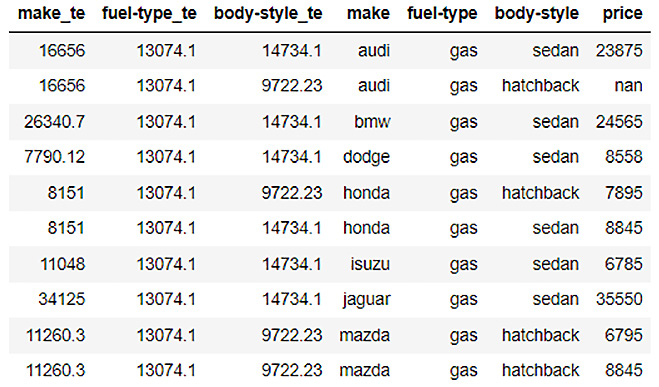
Figure 3.34 – An encoded automobile price prediction test dataframe

As you can see from the figure, our test frame also has three additional columns, which are the encoded columns. You can now use these dataframes to train your ML models.

Depending on your next actions, you can use the encoded dataframes however you see fit. If you want to use the dataframe to train ML models, then you can drop the categorical columns from the dataframe and use the respective encoded columns as training features to train your models. If you wish to perform any further analytics on the dataset, then you can keep both types of columns and perform any comparative study.

Tip

H2O’s target encoder has several parameters that you can set to tweak the encoding process. Selecting the correct settings for target encoding your dataset can get very complex, depending on the type of data with which you are working. So, feel free to experiment with this function, as the better you understand this feature and target encoding in general, the better you can encode your dataframe and further improve your model training. You can find more details about H2O’s target encoder here: https://docs.h2o.ai/h2o/latest-stable/h2o-docs/data-science/target-encoding.html.

Congratulations! You have just understood how you can encode categorical values using H2O’s target encoder.

Summary

In this chapter, we first explored the various techniques and some of the common functions we use to preprocess our dataframe before it is sent to model training. We looked into how we can reframe our raw dataframe into a suitable consistent format that meets the requirement for model training. We learned how to manipulate the columns of dataframes by combining them with different columns of different dataframes. We learned how to combine rows from partitioned dataframes, as well as how to directly merge dataframes into a single dataframe.

Once we knew how to reframe our dataframes, we learned how to handle the missing values that are often present in freshly collected data. We learned how to fill NA values, replace certain incorrect values, as well as how to use different imputation strategies to avoid adding noise and bias when filling missing values.

We then investigated how we can manipulate the feature columns by sorting the dataframes by column, as well as changing the types of columns. We also learned how to tokenize strings to handle textual data, as well as how to encode categorical values using H2O’s target encoder.

In the next chapter, we will open the black box of AutoML, explore its training, and what happens internally during the AutoML process. This will help us to better understand how H2O does its magic and efficiently automates the model training process.