TensorFlow.js is an open source JavaScript library for machine learning. It is developed by Google and is a companion library to TensorFlow, in Python.
This tool enables you to build machine learning applications that can run in the browser or in Node.js.
This way, users don’t need to install any software or driver. Simply opening a web page allows you to interact with a program.
2.1 Basics of TensorFlow.js
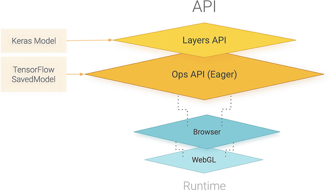
Visual representation of the TensorFlow.js API. Source: https://blog.tensorflow.org/2018/03/introducing-tensorflowjs-machine-learning-javascript.html
It also supports importing models saved from TensorFlow and Keras.
At the core of TensorFlow is tensors. A tensor is a unit of data, a set of values shaped into an array of one or more dimensions. It is similar to multidimensional arrays.
2.1.1 Creating tensors
Example of 2D array
Creating a tensor out of an array
Now, the variable dataTensor can be used with other TensorFlow methods to train a model, generate predictions, and so on.
rank: Indicates how many dimensions the tensor contains
shape: Defines the size of each dimension of the data
dtype: Defines the data type of the tensor
Logging a tensor’s shape, rank, and dtype
In the sample tensor illustrated, the shape returns [3, 3] as we can see 3 arrays containing 3 values.
The rank property prints 2 as we are working with a 2D array. If we had added another dimension to our array, the rank would have been 3.
Finally, the dtype is float32 as this is the default data type.
Creating different kinds of tensors
In the sample code shown so far, we used tf.tensor to create tensors; however, more methods are available to create them with different dimensions.
Depending on the data you are working with, you can use the methods from tf.tensor1d to tf.tensor6d to create tensors of up to six dimensions.
Creating multidimensional tensors
Creating tensors from flat arrays
Once a tensor has been instantiated, it is possible to change its shape using the reshape method.
2.1.2 Accessing data in tensors
Once a tensor is created, you can get its values using tf.array() or tf.data().
Accessing data in tensors
As you can see in the preceding example, these two methods return a promise.
In JavaScript, a promise is a proxy for a value that is not created yet at the time the promise is called. Promises represent operations that have not completed yet, so they are used with asynchronous actions to supply a value at some point in the future when the action has completed.
Accessing data in tensors synchronously
It is not recommended to use them in production applications as they will cause performance issues.
2.1.3 Operations on tensors
In the previous section, we learned that tensors are data structures that allow us to store data in a way TensorFlow.js can work with. We saw how to create them, shape them, and access their values.
Now, let’s look into some of the different operations that allow us to manipulate them.
These operations can be organized into categories. Some of them allow you to do arithmetic on a tensor, for example, adding multiple tensors together, other operations focus on doing logical operations such as evaluating if a tensor is greater than another, and others provide a way to do basic maths, like computing the square of all elements in a tensor.
The full list of operations is available at https://js.tensorflow.org/api/latest/#Operations.
Example of operation on a tensor
In this example, we’re adding two tensors together. If you’re looking at the first value of tensorA, which is 1, and the first value of tensorB, which is 5, adding 1 + 5 does result in the number 6, which is the first value of our final tensor.
To be able to use this kind of operations, your tensors have to have the same shape but not necessarily the same rank.
If you remember from the last few pages, the shape is the amount of values in each dimension of the tensor, when the rank is the amount of dimensions.
Example of operation on a tensor
In this case, tensorA is now a 2D tensor, but tensorB is still one dimensional.
The result of adding the two is now a tensor with the same values as before but with a different number of dimensions.
Error generated when using an incorrect shape
What this error is telling us is that this operand cannot be used with these two tensors, as one of them has four elements, and the other only three.
Tensors are immutable, so these operations will not mutate the original tensors, but will instead always return a new tf.Tensor.
2.1.4 Memory
Using the dispose method
Another way to manage memory is using tf.tidy() when chaining operations.
Using the tidy method
In this example, the result of square() is going to be disposed, whereas the result of neg() won’t as it returns the value of the function.
Now that we have covered what is at the core of TensorFlow.js and how to work with tensors, let’s look into the different features offered by the library to get a better idea of what is possible.
2.2 Features
In this subchapter, we are going to explore the three main features currently available in TensorFlow.js. This includes using a pre-trained model; doing transfer learning, which means retraining a model with custom input data; and doing everything in JavaScript, meaning, creating a model, training it, and running predictions, all in the browser.
We will cover these features from the simplest to use to the most complex.
2.2.1 Using a pre-trained model
In the first chapter of this book, we defined the term “model” as a mathematical function that can take new parameters to make predictions based on the data it had been trained with.
If this definition is still a bit confusing to you, hopefully putting it into context while talking about this first feature is going to make it a bit clearer.
In machine learning, to be able to predict an outcome, we need a model. However, it is not necessary to have built the model yourself. It is totally fine to use what is called “pre-trained models.”
The term “pre-trained” means that this model has already been trained with a certain type of input data and has been developed for a specific purpose.
For example, you can find some open source pre-trained models focused on object detection and recognition. These models have already been fed with millions of images of objects, have gone through all the training process, and should now have a satisfying level of accuracy when predicting new entities.
Companies or institutions creating these models make them open source so developers can use them in their application and have the opportunity to build machine learning projects much faster.
As you can imagine, the process of gathering data, formatting it, labelling it, experimenting with different algorithms and parameters can take a lot of time, so being able to substitute this work by using a pre-trained model frees up a lot of time to focus on building applications.
Pre-trained models currently available to use with TensorFlow.js include body segmentation, pose estimation, object detection, image classification, speech command recognition, and sentiment analysis.
Using a pre-trained model in your application is relatively easy.
Classifying an image using the mobilenet model
In a real application, this code would need to require the TensorFlow.js library and mobilenet pre-trained model beforehand, but more complete code samples will be shown in the next few chapters as we dive into building actual projects.
The preceding sample starts by getting the HTML element that should contain the image we would like to predict. The next step is to load the mobilenet model asynchronously.
Models can be of a rather large size, sometimes a few megabytes, so they need to be loaded using async/await to make sure that this operation is fully finished by the time you run the prediction.
Once the model is ready, you can call the classify() method on it, in which you pass your HTML element, that will return an array of predictions.

A picture of a cat

Result of the image classification from the mobilenet model applied to the picture of the cat earlier
The result of using classify() is always an array of three objects containing two keys: className and probability.
The className is a string containing the label, or class, the model has categorized the new input in, based on the data it has been previously trained with.
The probability is a float value between 0 and 1 that represents the likelihood of the input data belonging to the className, 0 being not likely and 1 being very likely.
They are organized in descending order so the first object in the array is the prediction the most likely to be true.
In the output earlier, the model predicts that the image contains a “tiger cat” with 70% likelihood.
The rest of the predictions have a probability value that drops quite significantly, with 21% chance that it contains a “tabby cat” and about 0.02% probability that it contains a “bow tie.”
In general, you would focus on the first value returned in the predictions, as it has the highest probability; however, 70% is actually not that high.
In machine learning, you aim to have the highest probability possible when using predictions. In this case, we only predicted the existence of a cat in an image, but in real applications, you can imagine that a 30% chance of having predicted an incorrect output is not acceptable.
To improve this, in general, we would do what is called “hyperparameter tuning ” and retrain the model.
Hyperparameter tuning is the process of tweaking and optimizing the parameters used when generating a model. It could be adding layers in a neural network, changing the batch size, and so on and seeing the effect of these changes on the performance and accuracy of the model.
However, when using a pre-trained model, you would not have the ability to do this, as the only thing you have access to is the output model, not the code written to create it.
This is one of the limits that comes with using pre-trained models.
When using these models, you have no control over how they were created and how to modify them. You usually don’t have access to the dataset used in the training process, so you cannot be sure that it will meet the requirements for your application.
Besides, you take the risk of inheriting the company’s or institution’s biases.
If your application involves implementing facial recognition and you decide to use an open source pre-trained model, you cannot be sure this model was trained on a diverse dataset of people. As a result, you may be unknowingly supporting certain biases by using them.
There had been issues in the past with facial recognition models only performing well on white people, leaving behind a huge group of users with darker skin.
Even though work has been done to fix this, we regularly hear about machine learning models making biased predictions because the data used to train them was not diverse enough.
If you decide to use a pre-trained model in a production application, I believe it’s important to do some research beforehand.
2.2.2 Transfer learning
The second feature available in TensorFlow.js is called “transfer learning .”
Transfer learning is the ability to reuse a model developed for a task, as the starting point for a model on a second task.
If you imagine an object recognition model that has been pre-trained on a dataset you don’t have access to, the function at the core of the model is to recognize entities in images. Using transfer learning, you can leverage this model to create a new one which function will be the same, but trained using your custom input data.
Transfer learning is a way to generate a semicustomized model. You are still not able to modify the model itself, but you can feed it your own data, which can improve the accuracy of the predictions.
If we reuse our example from the previous section where we used a pre-trained model to detect the presence of a cat in a picture, we could see that the prediction came back with the label “tiger cat.” This means that the model was trained with images labelled as such, but what if we want to detect something very different, like Golden Wattles (Australian flowers)?
The first step would be to search for the list of classes the model can predict and see if it contains these flowers. If it does, it means the model can be used directly, just like shown in the previous section.
However, if it was not trained with images of Golden Wattles, it will not be able to detect them until we generate a new model using transfer learning.
To do this, a part of the code is similar to the samples shown in the previous section as we still need to start with the pre-trained model, but we introduce some new logic.
Importing TensorFlow.js, mobilenet, and a KNN classifier
Doing so gives us access to a knnClassifier object.
Instantiating the KNN classifier
This classifier is going to be used to enable us to make predictions from custom input data, instead of only using the pre-trained model.
Adding example data to a KNN classifier
The preceding code sample is incomplete, but we will cover it more in depth in the following chapters, when we focus on implementing transfer learning in an application.
The most important here is to understand that we save an image from the webcam feed in a variable, use it as new data on the model, and add this as an example with a class (label) to the classifier, so the end result is a model that is able to recognize not only the data similar to the one used in the initial training process of the mobilenet model but also our new samples.
Feeding a single new image and example to the classifier is not enough for it to be able to accurately recognize our new input data; therefore, this step has to be repeated multiple times.
Classifying a new image
The first steps are the same, but instead of adding the example to the classifier, we use the predictClass method to return a result of what it thinks the new input is.
We will go more in depth about transfer learning in the next chapter.
2.2.3 Creating, training, and predicting
Finally, the third feature allows you to create the model yourself, run the training process, and use it, all in JavaScript.
This feature is more complex than the two previous ones but will be covered more deeply in Chapter 5, when we build an application using a model we will create ourselves.
It is important to know that creating a model yourself requires a trial and error approach.
There is not a single way to solve a problem, and if you decide to go down that path, you will need to experiment a lot with different algorithms, parameters, and so on.
The most common type of model used is a sequential model that you can create with a list of layers.
Creating a model
We start by instantiating it using tf.sequential and add multiple different layers to it.
This step is a bit arbitrary in the sense that choosing the type and number of layers, as well as the parameters passed to the layers, is more of an art than a science.
Your model will probably not be perfect the first time you write it and will require multiple changes before you end up with a result that will be the most performant.
One important thing to keep in mind is to provide an inputShape parameter in the first layer of your model to indicate the shape of the data the model is going to be trained on. The subsequent layers do not need it.
Fitting a model with data
In general, before calling this method, you split your data into batches to train your model little by little. An entire dataset is often too big to be used at once, so dividing it into batches is important.
The options parameter passed into the function is an object containing information about the training process. You can specify the number of epochs, which is when the entire dataset is passed through the neural network, and also the batch size, which represents the number of training examples present in a single batch.
As the dataset is split up in batches passed in the fit method, we also need to think about the number of iterations needed to train the model with the full dataset.
For example, if our dataset contains 1000 examples and our batch size is 100 examples at a time, it will take 10 iterations to complete 1 epoch.
Therefore, we will need to loop and call our fit method 10 times, updating the batched data each time.
Predicting
There is more to cover about this feature, but we will look into it further with our practical example in the next few chapters.