1
Introduction to Quantum Mechanics
- 1.1 Introduction
- 1.2 The Classical Electron
- 1.3 Two Slit Electron Experiment
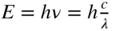
- 1.4 The Photoelectric Effect
- 1.5 Wave Packets and Uncertainty
- 1.6 The Wavefunction
- 1.7 The Schrödinger Equation
- 1.8 The Electron in a One‐Dimensional Well
- 1.9 Electron Transmission and Reflection at Potential Energy Step
- 1.10 Expectation Values
- 1.11 Spin
- 1.12 The Pauli Exclusion Principle
- 1.13 Summary
- Further Reading
- Problems
1.1 Introduction
The study of semiconductor devices relies on the electronic properties of solid‐state materials and hence a fundamental understanding of the behaviour of electrons in solids.
Electrons are responsible for electrical properties and optical properties in metals, insulators, inorganic semiconductors, and organic semiconductors. These materials form the basis of an astonishing variety of electronic components and devices. Among these, devices based on the p–n junction are of key significance and they include solar cells and light‐emitting diodes (LEDs) as well as other diode devices and transistors.
The electronics age in which we are immersed would not be possible without the ability to grow these materials, control their electronic properties, and finally fabricate structured devices using them, which yield specific electronic and optical functionality.
Electron behaviour in solids requires an understanding of the electron that includes the quantum mechanical description; however, we will start with the classical electron.
1.2 The Classical Electron
We describe the electron as a particle having mass
and negative charge of magnitude
If an external electric field ε(x, y, z) is present in three‐dimensional space and an electron experiences this external electric field, the magnitude of the force on the electron is
The direction of the force is opposite to the direction of the external electric field due to the negative charge on the electron. If ε is expressed in volts per meter (V m−1 ) then F will have units of newtons.
If an electron accelerates through a distance d from point A to point B in vacuum due to a uniform external electric field ε , it will gain kinetic energy ΔE in which
This kinetic energy ΔE gained by the electron may be expressed in Joules within the Meter–Kilogram–Second (MKS) unit system. We can also say that the electron at point A has a potential energy U that is higher than its potential energy at point B. Since total energy is conserved,
There exists an electric potential V(x, y, z) defined in units of the volt at any position in three‐dimensional space associated with an external electric field. We obtain the spatially dependent potential energy U(x, y, z) for an electron in terms of this electric potential from
We also define the electron‐volt, another commonly used energy unit. By definition, one electron‐volt in kinetic energy is gained by an electron if the electron accelerates in an electric field between two points in space whose difference in electric potential ΔV is 1 V.
If an external magnetic field B is present, the force on an electron depends on the charge q on the electron as well as the component of electron velocity v perpendicular to the magnetic field, which we shall denote as v ⊥ . This force, called the Lorentz Force, may be expressed as F = −q( v ⊥ × B ). The force is perpendicular to both the velocity component of the electron and to the magnetic field vector. The Lorentz force is the underlying mechanism for the electric motor and the electric generator.
This classical description of the electron generally served the needs of the vacuum tube electronics era and the electric motor/generator industry in the first half of the twentieth century.
In the second half of the twentieth century, the electronics industry migrated from vacuum tube devices to solid‐state devices once the transistor was invented at Bell Laboratories in 1954. The understanding of the electrical properties of semiconductor materials from which transistors are made could not be achieved using a classical description of the electron. Fortunately, the field of quantum mechanics, which was developing over the span of about 50 years before the invention of the transistor, allowed physicists to model and understand electron behaviour in solids.
In this chapter we will motivate quantum mechanics by way of a few examples. The classical description of the electron is shown to be unable to explain some simple observed phenomena, and we will then introduce and apply the quantum‐mechanical description that has proven to work very successfully.
1.3 Two Slit Electron Experiment
One of the most remarkable illustrations of how strangely electrons can behave is illustrated in Figure 1.1. Consider a beam of electrons arriving at a pair of narrow, closely spaced slits formed in a solid. Assume that the electrons arrive at the slits randomly in a beam having a width much wider than the slit dimensions. Most of the electrons hit the solid, but a few electrons pass through the slits and then hit a screen placed behind the slits as shown.
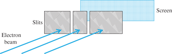
Figure 1.1 Electron beam emitted by an electron source is incident on narrow slits with a screen situated behind the slits
If the screen could detect where the electrons arrived by counting them, we would expect a result as shown in Figure 1.2.

Figure 1.2 Classically expected result of two‐slit experiment
In practice, a screen pattern as shown in Figure 1.3 is obtained. This result is impossible to derive using the classical description of an electron.

Figure 1.3 Result of two‐slit experiment. Notice that a wave‐like electron is required to cause this pattern. If light waves rather than electrons were used, then a similar plot would result except the vertical axis would be a measure of the light intensity instead
It does become readily explainable, however, if we assume the electrons have a wave‐like nature. If light waves, rather than particles, are incident on the slits, then there are particular positions on the screen at which the waves from the two slits cancel out. This is because they are out of phase. At other positions on the screen the waves add together because they are in‐phase. This pattern is the well‐known interference pattern generated by light travelling through a pair of slits. Interestingly we do not know which slit a particular electron passes through. If we attempt to experimentally determine which slit an electron is passing through we immediately disrupt the experiment and the interference pattern disappears. We could say that the electron somehow goes through both slits. Remarkably, the same interference pattern builds up slowly and is observed even if electrons are emitted from the electron source and arrive at the screen one at a time. We are forced to interpret these results as a very fundamental property of small particles such as electrons.
We will now look at how the two‐slit experiment for electrons may actually be performed. It was done in the 1920s by Davisson and Germer. It turns out that very narrow slits are required to be able to observe the electron behaving as a wave due to the small wavelength of electrons. Fabricated slits having the required very small dimensions are not practical, but Davisson and Germer realised that the atomic planes of a crystal can replace slits. By a process of electron reflection, rows of atoms belonging to adjacent atomic planes on the surface of a crystal act like tiny reflectors that effectively form two beams of reflected electrons that then reach a screen and form an interference pattern similar to that shown in Figure 1.3.
Their method is shown in Figure 1.4. The angle between the incident electron beam and each reflected electron beam is θ . The spacing between surface atoms belonging to adjacent atomic planes is d . The path length difference between the two beam paths shown is d sin θ . A maximum on the screen is observed when
or an integer number of wavelengths. Here, n is an integer and λ is the wavelength of the waves. A minimum occurs when
which is an odd number of half wavelengths causing wave cancellation.

Figure 1.4
Davisson–Germer experiment showing electrons reflected off adjacent crystalline planes. Path length difference is 
In order to determine the wavelength of the apparent electron wave we can solve Eq. 1.2a and 1.2b for λ . We have the appropriate values of θ ; however, we need to know d. Using X‐ray diffraction and Bragg's law we can obtain d. Note that Bragg's law is also based on wave interference except that the waves are X‐rays.
The results that Davisson and Germer obtained were quite startling. The calculated values of
λ
were on the order of angstroms, where 1 ![]() is one‐tenth of a nanometre. This is much smaller than the wavelength of light, which is on the order of thousands of angstroms, and it explains why regular slits used in optical experiments are much too large to observe electron waves. But more importantly the measured values of
λ
actually depended on the incident velocity
v
or momentum
mv
of the electrons used in the experiment. Increasing the electron momentum by accelerating electrons through a higher potential difference before they reached the crystal caused
λ
to decrease, and decreasing the electron momentum caused
λ
to increase. By experimentally determining
λ
for a range of values of incident electron momentum, the following relationship was discovered:
is one‐tenth of a nanometre. This is much smaller than the wavelength of light, which is on the order of thousands of angstroms, and it explains why regular slits used in optical experiments are much too large to observe electron waves. But more importantly the measured values of
λ
actually depended on the incident velocity
v
or momentum
mv
of the electrons used in the experiment. Increasing the electron momentum by accelerating electrons through a higher potential difference before they reached the crystal caused
λ
to decrease, and decreasing the electron momentum caused
λ
to increase. By experimentally determining
λ
for a range of values of incident electron momentum, the following relationship was discovered:
This is known as the de Broglie equation, because de Boglie postulated this relationship before it was validated experimentally. Here
p
is the magnitude of electron momentum, and
h = 6.63 × 10⁻³⁴ Js is a constant known as Planck's constant. In an alternative form of the equation we define ![]() , pronounced h‐bar to be
, pronounced h‐bar to be ![]() and we define
k
, the wavenumber to be
and we define
k
, the wavenumber to be ![]() . Now we can write the de Broglie equation as
. Now we can write the de Broglie equation as
Note that p is the magnitude of the momentum vector p and k is the magnitude of wavevector k . The significance of wavevectors will be made clear in Chapter 2.
1.4 The Photoelectric Effect
About 30 years before Davisson and Germer discovered and measured electron wavelengths, another important experiment had been undertaken by Heinrich Hertz. In 1887, Hertz was investigating what happens when light is incident on a metal. He found that electrons in the metal can be liberated by the light. It takes a certain amount of energy to release an electron from a metal into vacuum. This energy is called the workfunction Φ, and the magnitude of Φ depends on the metal.
If the metal is placed in a vacuum chamber, the liberated electrons are free to travel away from the metal and they can be collected by a collector electrode also located in the vacuum chamber shown in Figure 1.5. This is known as the photoelectric effect.
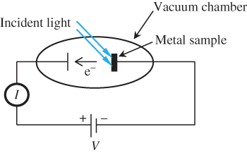
Figure 1.5
The photoelectric experiment. The current  flowing through the external circuit is the same as the vacuum current
By carefully measuring the resulting electric current I flowing through the vacuum, scientists in the last decades of the nineteenth century were able to make the following statements:
- The electric current increases with increasing light intensity.
- The colour or wavelength of the light is also important. If monochromatic light is used, there is a particular critical wavelength above which no electrons are released from the metal even if the light intensity is increased.
- This critical wavelength depends on the type of metal employed. Metals composed of atoms having low ionisation energies such as cerium and calcium have larger critical wavelengths. Metals composed of atoms having higher ionisation energies such as gold or aluminium require smaller critical wavelengths.
- If light having a wavelength equal to the critical wavelength is used, then the electrons leaving the metal surface have no initial kinetic energy and collecting these electrons requires that the voltage V must be positive to accelerate the electrons away from the metal and towards the second electrode.
- If light having wavelengths smaller than the critical wavelength is used then the electrons do have some initial kinetic energy. Now, even if V is negative so as to retard the flow of electrons from the metal to the electrode, some electrons may be collected. There is, however, a maximum negative voltage of magnitude V max for which electrons may be collected. As the wavelength of the light is further decreased, V max increases (the maximum voltage becomes more negative).
- If very low intensity monochromatic light with a wavelength smaller than the critical wavelength is used then individual electrons are measured rather than a continuous electron current. Suppose at time t = 0 there is no illumination, and then at time t > 0 very low intensity light is turned on. The first electron to be emitted may occur virtually as soon as the light is turned on, or it may take a finite amount of time to be emitted after the light is turned on. There is no way to predict this amount of time in advance.
Einstein won the Nobel Prize for his conclusions based on these observations. He concluded the following:
- Light is composed of particle‐like entities or wave packets commonly called photons.
- The intensity of a source of light is determined by the photon flux density, or the number of photons being emitted per second per unit area.
- Electrons are emitted only if the incident photons each have enough energy to overcome the metal's workfunction.
- The photon energy of an individual photon of monochromatic light is determined by the colour (wavelength) of the light.
- Photons of a known energy are randomly emitted from monochromatic light sources, and we can never precisely know when the next photon will be emitted.
- Normally we do not notice these photons because there are a very large number of photons in a light beam. If, however, the intensity of the light is low enough, then the photons become noticeable and light becomes granular.
- If light having photon energy larger than the energy needed to overcome the workfunction is used, then the excess photon energy causes a finite initial kinetic energy of the escaped electrons.
By carefully measuring the critical photon wavelength λ c as a function of V max , the relationship between photon energy and photon wavelength can be determined: The initial kinetic energy E k of the electron leaving the metal can be sufficient to overcome a retarding (negative) potential difference V between the metal and the electrode. Since the kinetic energy lost by the electron as it moves against this retarding potential difference V is E k = |qV|, we can deduce the minimum required photon energy E using the energy equation E = Φ + qV max . This experimentally observed relationship is
where c is the velocity of light. Since the frequency of the photon ν is given by
we obtain the following relationship between photon energy and photon frequency:
where ω = 2πν . Note that Planck's constant h is found when looking at either the wave‐like properties of electrons in Eq. (1.3) or the particle‐like properties of light in Eq. 1.4. This wave‐particle duality forms the basis for quantum mechanics.
Equation 1.4 that arose from the photoelectric effect defines the energy of a photon. In addition, Eq. (1.3) that arose from the Davisson and Germer experiment applies to both electrons and photons. This means that a photon having a known wavelength carries a specific momentum ![]() even though a photon has no mass. The existence of photon momentum is experimentally proven since light‐induced pressure can be measured on an illuminated surface.
even though a photon has no mass. The existence of photon momentum is experimentally proven since light‐induced pressure can be measured on an illuminated surface.
In summary, electromagnetic waves exist as photons, which also have particle‐like properties such as momentum and energy, and particles such as electrons also have wave‐like properties such as wavelength.
1.5 Wave Packets and Uncertainty
Uncertainty in the precise position of a particle is embedded in its quantum mechanical wave description. The concept of a wave packet introduced in Section 1.4 for light is important since it is applicable to both photons and particles such as electrons.
A wave packet is illustrated in Figure 1.6 showing that the wave packet has a finite size. A wave packet can be analysed into, or synthesised from, a set of component sinusoidal waves, each having a distinct wavelength, with phases and amplitudes such that they interfere constructively only over a small region of space to yield the wave packet, and destructively elsewhere. This set of component sinusoidal waves of distinct wavelengths added to yield an arbitrary function is a Fourier series.
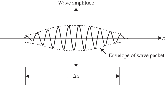
Figure 1.6 Wave packet. The envelope of the wave packet is also shown. More insight about the meaning of the wave amplitude for a particle such as an electron will become apparent in Section 1.6 in which the concept of a probability amplitude is introduced
The uncertainty in the position of a particle described using a wave packet may be approximated as Δx as indicated in Figure 1.6. The uncertainty depends on the number of component sinusoidal waves being added together in a Fourier series: If only one component sinusoidal wave is present, the wave packet is infinitely long, and the uncertainty in position is infinite. In this case, the wavelength of the particle is precisely known, but its position is not defined. As the number of component sinusoidal wave components of the wave packet approaches infinity, the uncertainty Δx of the position of the wave packet may drop and we say that the wave packet becomes increasingly localised.
An interesting question now arises: If the wave packet is analysed into, or composed from, a number of component sinusoidal waves, can we define the precise wavelength of the wave packet? It is apparent that as more component sinusoidal waves, each having a distinct wavelength, are added together the uncertainty of the wavelength associated with the wave packet will become larger. From Eq. (1.3), the uncertainty in wavelength results in an uncertainty in momentum p and we write this momentum uncertainty as Δp .
By doing the appropriate Fourier series calculation, (see Appendix 2) the relationship between Δx and Δp can be shown to satisfy the following condition:
As Δx is reduced, there will be an inevitable increase in Δp. This is known as the Uncertainty Principle. We cannot precisely and simultaneously determine the position and the momentum of a particle. If the particle is an electron we know less and less about the electron's momentum as we determine its position more and more precisely.
Since a photon is also described in terms of a wave packet, the concept of uncertainty applies to photons as well. As the location of a photon becomes more precise, the wavelength or frequency of the photon becomes less well defined. Photons always travel with velocity of light
c
in vacuum. The exact arrival time
t
of a photon at a specific location is uncertain due to the uncertainty in position. For the photoelectric effect described in Section 1.4, the exact arrival time of a photon at a metal was observed not to be predictable for the case of monochromatic photons for which ![]() is accurately known. If we allow some uncertainty in the photon frequency
Δω
the energy uncertainty
ΔE =
is accurately known. If we allow some uncertainty in the photon frequency
Δω
the energy uncertainty
ΔE =
![]() Δω
of the photon becomes finite, but then we can know more about the arrival time. The resulting relationship that may be calculated by the same approach as presented in Appendix 2 may be written as
Δω
of the photon becomes finite, but then we can know more about the arrival time. The resulting relationship that may be calculated by the same approach as presented in Appendix 2 may be written as ![]() . This type of uncertainty relationship is useful in time‐dependent problems and, like the derivation of uncertainty for particles such as electrons, it results from a Fourier transform: The frequency spectrum Δω
of a pulse in the time domain becomes wider as the pulse width Δt
becomes narrower.
. This type of uncertainty relationship is useful in time‐dependent problems and, like the derivation of uncertainty for particles such as electrons, it results from a Fourier transform: The frequency spectrum Δω
of a pulse in the time domain becomes wider as the pulse width Δt
becomes narrower.
A wave travels with velocity v = fλ = ω/k . Note that we refer to this as a phase velocity because it refers to the velocity of a point on the wave that has a given phase, for example the crest of the wave. For a travelling wave packet, however, the velocity of the particle described using the wave packet is not necessarily the same as the phase velocity of the individual waves making up the wave packet. The velocity of the particle is actually determined using the velocity of the wave‐packet envelope shown in Figure 1.6. The velocity of propagation of this envelope is called the group velocity v g because the envelope is formed by the Fourier sum of a group of waves.
When photons travel through media other than vacuum, dispersion can exist. Consider the case of a photon having energy uncertainty
ΔE =
![]() Δω
due to its wave‐packet description. In the case of this photon travelling through vacuum, the group velocity and the phase velocity are identical to each other and equal to the speed of light
c
. This is known as a dispersion‐free photon for which the wave packet remains intact as it travels. But if a photon travels through a medium other than vacuum there is often finite dispersion in which some Fourier components of the photon wave packet travel slightly faster or slightly slower that other components of the wave packet, and the photon wave packet broadens spatially as it travels. For example, photons travelling through optical fibres typically suffer dispersion, which limits the ultimate temporal resolution of the fibre system.
Δω
due to its wave‐packet description. In the case of this photon travelling through vacuum, the group velocity and the phase velocity are identical to each other and equal to the speed of light
c
. This is known as a dispersion‐free photon for which the wave packet remains intact as it travels. But if a photon travels through a medium other than vacuum there is often finite dispersion in which some Fourier components of the photon wave packet travel slightly faster or slightly slower that other components of the wave packet, and the photon wave packet broadens spatially as it travels. For example, photons travelling through optical fibres typically suffer dispersion, which limits the ultimate temporal resolution of the fibre system.
It is very useful to plot ω versus k for the given medium in which the photon travels. If a straight line is obtained then v = ω/k is a constant and the velocity of each Fourier component of the photon's wave packet is identical. This is dispersion‐free propagation. In general, however, a straight line will not be observed and dispersion exits.
In Appendix 3 we analyse the velocity of a wave packet composed of a series of waves. It is shown that the wave packet travels with velocity
This is valid for both photons and particles such as electrons. For wave packets of particles, however, we can further state that
This relationship will be important in Chapter 2 to determine the velocity of electrons in crystalline solids.
1.6 The Wavefunction
Based on what we have observed up to this point, the following four points more completely describe the properties of an electron in contrast to the description of the classical electron of Section 1.2:
- The electron has mass m .
- The electron has charge q .
- The electron has wave properties with wavelength
 .
. - The exact position and momentum of an electron cannot be measured simultaneously.
Quantum mechanics provides an effective mathematical description of particles such as electrons that was motivated by the above observations. A wavefunction ψ is used to describe the particle and ψ may also be referred to as a probability amplitude. In general, ψ is a complex number, which is a function of space and time. Using Cartesian spatial coordinates, ψ = ψ(x, y, z, t). We could also use other coordinates such as spherical polar coordinates in which case we would write ψ = ψ(r, θ, φ, t).
The use of complex numbers is very important for wavefunctions because it allows them to represent waves as will be seen in Section 1.7.
Although ψ is a complex number and is therefore not a real, measurable or observable quantity, the quantity ψ * ψ = |ψ|2 where ψ * is the complex conjugate of ψ , is an observable and must be a real number. |ψ|2 is referred to as a probability density. At any time t , using cartesian coordinates, the probability of the particle being in volume element dx dy dz at location (x, y, z) will be |ψ(x, y, z)|2dx dy dz . If a particle exists, then it must be somewhere in space and we can write
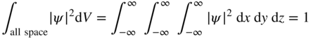
The wavefunction, therefore, fundamentally recognises the attribute of uncertainty and simultaneously is able to represent a wave. We cannot precisely define the position of the particle; however, we can determine the probability of it being in a specific region. Equation 1.6 is referred to as the normalisation condition for a wavefunction and a wavefunction that satisfies this equation is a normalised wavefunction.
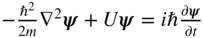
1.7 The Schrödinger Equation
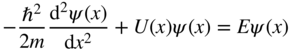
In order to give the particle we are trying to describe the attributes of a wave, the form of ψ may be a mathematical wave expression such as the sinusoidal function used in Example 1.4. Building on the emerging understanding of particles we have outlined in this chapter and through the remarkable insights of Erwin Schrödinger, in 1925 the following wave equation, called the Schrödinger equation, was postulated:
U(x, y, z) represents the potential energy in the electric field in which the particle of mass m exists and the equation allows the particle's wavefunction ψ (x, y, z, t) to be found. The first term is associated with the kinetic energy of the particle. The second term is associated with the potential energy of the particle, and the right‐hand side of the equation is associated with the total energy E of the particle. Once ψ is known, the particle's position, energy, and momentum can be determined either as specific values or as spatial distribution functions consistent with the uncertainty principle. For time‐varying systems, a possible time evolution of the particle's properties may also be described.
Although this equation is applicable to particles including electrons and protons, we are interested in the electrical properties of materials and we will therefore focus on the electron. By solving Schrödinger's equation for an electron in a few simple scenarios, we will be able to appreciate the utility of the equation as well as the quantum mechanical wavefunction‐based description of the electron.
Let us propose a solution to Eq. 1.7 having the form:
Note that we have separated the solution into two parts, one for spatial dependence and one for time dependence. Now substituting Eq. 1.8 into Eq. 1.7 and dividing by ψ(x, y, z)T(t) we obtain:

Since the left side is a function of independent variables x, y, z only and the right side is a function of independent variable t only, the only way for the equality to hold for both arbitrary spatial locations and arbitrary moments in time is for both sides of the equation to be equal to a constant that we will call E.
The resulting equations are:
and
Equations 1.9 and 1.10 are the result of the just‐described method known as the separation of variables applied to Eq. 1.7. Equation 1.9 is easy to solve and has solution
If we now identify E with the energy of the electron and use Eq. 1.4 we obtain
and therefore
which represents the expected time‐dependence of a wave having frequency ω .
Equation 1.10 is known as the Time‐Independent Schrödinger Equation and it is useful for a wide variety of steady‐state (time‐independent) situations as illustrated in Examples 1.5–1.8.
1.8 The Electron in a One‐Dimensional Well
In practical situations, electrons are not free to move infinite distances along an axis and we will now consider the case of an electron that is free to move over a finite portion of the x‐axis only. Beyond this range the electron will encounter potential barriers that limit its movement.
Consider a one‐dimensional steady state or time‐invariant problem in which an electron is free to move around in the one‐dimensional potential well illustrated in Figure 1.7. The potential energy of an electron is zero inside the well and Φ outside the well. This model can be thought of in the context of a hypothetical solid having one dimension a with vacuum outside the solid. The electron potential energy is zero inside the solid and the height of the potential well is equal to the workfunction Φ of the solid.

Figure 1.7
Potential well with zero potential for  and a potential energy of Φ for
  or
or  . In a hypothetical solid we can consider the wall height of the well to be equal to the workfunction of the solid
To determine the wavefunctions of the electron, we again make use of the time‐independent Schrödinger equation 1.10
Inside the well, U = 0 and hence

The general solution of this from Eq. 1.13 is
ψ(x) = αe
ikx
+ βe−ikx
with ![]() . Note that these terms represent components of travelling waves moving in opposite directions. Since there is no preferred travelling wave direction due to the symmetry of the potential well about the origin, we can conclude that these waves form a standing wave, i.e. |α| = |β|. Since there is no time dependence, these solution are referred to as stationary states or eigenstates.
. Note that these terms represent components of travelling waves moving in opposite directions. Since there is no preferred travelling wave direction due to the symmetry of the potential well about the origin, we can conclude that these waves form a standing wave, i.e. |α| = |β|. Since there is no time dependence, these solution are referred to as stationary states or eigenstates.
There are two possibilities:
If α = β we obtain a symmetric function
or if α = − β we obtain an asymmetric function
Note that coefficient A is an imaginary number in Eq. 1.17b. This is not a difficulty since the observable |ψ|2 = ψ * ψ is always a real number.
In regions where the potential energy is equal to Φ we again apply Eq. 1.16. We will assume that the potential step in Figure 1.7 satisfies the condition Φ > E . Equation 1.16 may be written as:

Since (Φ − E) is positive, the general solution is
where
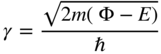
To further simplify
ψ(x), we note that for ![]() it follows that D = 0 to eliminate the physically impossible solution in which
ψ(x) rises exponentially as
x
goes more negative. Similarly for
it follows that D = 0 to eliminate the physically impossible solution in which
ψ(x) rises exponentially as
x
goes more negative. Similarly for ![]() it follows that
C = 0.
it follows that
C = 0.
Hence for ![]()
and for ![]() ,
,
We can now apply boundary conditions at ![]() and at
and at ![]() . These boundary conditions require that both the wavefunction
ψ
and its slope
. These boundary conditions require that both the wavefunction
ψ
and its slope ![]() are continuous at the boundaries. In the absence of this condition the second derivative of the wavefunction
are continuous at the boundaries. In the absence of this condition the second derivative of the wavefunction ![]() would become infinite and the Schrödinger equation could not be satisfied.
would become infinite and the Schrödinger equation could not be satisfied.
In the symmetric case, for
ψ
to be continuous at ![]() , we obtain, using Eqs. 1.17a and 1.18b,
, we obtain, using Eqs. 1.17a and 1.18b,
and for ![]() to be continuous at
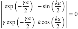
to be continuous at ![]() , by differentiating Eqs. 1.17a and 1.18b, we further obtain
, by differentiating Eqs. 1.17a and 1.18b, we further obtain
To obtain simultaneous solutions for D and A in Eq. (1.19), the determinant of the matrix formed from the coefficients must be zero. Thus,

This may be simplified to
Only discrete values of k and γ are allowed due to the periodicity of the tangent function.
In the asymmetric case for
ψ
to be continuous at ![]() we obtain, using Eqs. 1.17b and 1.18b,
we obtain, using Eqs. 1.17b and 1.18b,
and for ![]() to be continuous at
to be continuous at ![]() , by differentiating Eqs. 1.17b and 1.18b, we further obtain
, by differentiating Eqs. 1.17b and 1.18b, we further obtain
To obtain simultaneous solutions to D and A in Eqs. 1.21a and 1.21b the determinant of the matrix formed from the coefficients must be zero. Thus,
This may be simplified to
Again, only discrete values of k and γ are allowed.
An important limiting case of Example 1.9 is an infinite potential well for which Φ = ∞ (see Problem 1.6). This is used in Chapter 2 to develop the behaviour of electrons in semiconductors.
1.9 Electron Transmission and Reflection at Potential Energy Step
Consider now the influence of a potential step on the propagation of a beam of electrons. Figure 1.8 shows a potential step of height U 0 , which may be positive or negative. Let us assume that a beam of electrons with kinetic energy E > U 0 , moving from left to right, is incident upon the potential step at position x = 0.

Figure 1.8
(a) A beam of electrons with kinetic energy  moving from left to right is incident upon a potential step of height
  at
at  . A transmitted electron flux exists if
  . (b) If
  the condition
  is valid for all values of
The wavefunctions of the electrons are given by solutions of the time‐independent Schrödinger equation. For x ≤ 0,
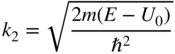
where

Wavefunctions ψ 2 will describe electrons that are transmitted across the step. Since the wavefunctions have energies E > U 0 we obtain
where
Since both
ψ
and ![]() must be continuous across the boundary at
x = 0 we can write
must be continuous across the boundary at
x = 0 we can write
or
and
or
Using Eqs. 1.25 and 1.26 the result can now be written as

and
Consider the electrons beam having wavefunction = Ae
ikx
. The flux of these electrons is proportional to the product of the probability density function and the electron momentum
p =
![]() k. We now define the reflection coefficient
R
as a ratio of fluxes between incident and reflected waves or
k. We now define the reflection coefficient
R
as a ratio of fluxes between incident and reflected waves or
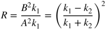
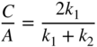
and the transmission coefficient T as a ratio of fluxes between incident and transmitted waves or

Note that R + T = 1 as expected.
The reflection coefficient R will approach 1 if k 1 ≪ k 2 or if k 2 ≪ k 1 . We will refer to these results when we describe electrons passing through potential barriers in semiconductor diode devices in Chapter 3.
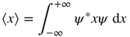
1.10 Expectation Values
Although there is uncertainty in the position of an electron in a one‐dimensional potential well, it is still possible to obtain an expected value of position for an electron. Since |ψ|2
is the probability density function we can determine the average value or expected value for the position of an electron by first normalising the wavefunction to ensure that ![]() . Then we can determine the expected value of the position
x
of the electron by conventional statistical methods regarding |ψ|2
as a distribution function and finding the average value of variable
x
by integrating the product |ψ|2
x
over the x‐axis. Hence we obtain
. Then we can determine the expected value of the position
x
of the electron by conventional statistical methods regarding |ψ|2
as a distribution function and finding the average value of variable
x
by integrating the product |ψ|2
x
over the x‐axis. Hence we obtain
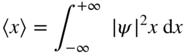
where 〈x〉 is used to denote the expectation value of variable x . Since |ψ|2 = ψ * ψ we can also write this using the complex conjugate of the wavefunction as
Using a common shorthand notation known as Dirac notation or bra‐ket notation we would write

It is also possible to determine expected values of other variables such as the expected value of momentum or energy of an electron. For example, the expected value of the momentum of the electron in the solutions to the Schrödinger equation in Example 1.9 is zero because the solutions originate from waves travelling in both directions with equal probabilities. A statistical treatment of all possible momentum values is required to obtain precise expectation values of momentum and textbooks devoted to quantum mechanics cover this. A related statistical treatment of all possible values is required to obtain precise values of uncertainty. Appendix 2 discusses this for the specific example of a Gaussian wave packet.
Expectation values will become important when we discuss the theory of radiation in Chapter 4.
1.11 Spin
Electrons and other particles possess another important characteristic called spin. In an experiment performed by Stern and Gerlach in the 1920s, a beam of silver atoms was evaporated from solid silver in a vacuum furnace and then passed through a magnetic field as shown in Figure 1.9. The magnetic field was a converging field in which the lines of magnetic field are more dense near one pole of the magnet.

Figure 1.9 The Stern–Gerlach experiment in which silver atoms are vaporised in a furnace and sent through a converging magnetic field. The north and south poles of the magnet have distinct shapes that give the field lines a higher density near the north pole
Consider a magnetic dipole caused by an orbiting electron. This is similar to the magnetic dipole formed by a current‐carrying wire in the shape of a coil wound around a core. In Figure 1.10 the silver atom is regarded as such a magnetic dipole. The converging field lines are also shown between the two distinctly shaped magnetic poles. A Lorentz force F = − q( v × B ) is directed outwards on the electron as it orbits. There is a component of this force F ⊥ that causes a net translational force on the magnetic dipole towards the upper magnet pole. If the magnetic field had no convergence then there would be no translational force.

Figure 1.10
A magnetic dipole formed by an orbiting electron passing through a converging magnetic field. The magnetic field causes a Lorentz force on the electron as shown in the detailed drawing on the right. For each electron position there is a force  that acts normal to the plane of electron orbit and towards the north pole of the magnet
Using silver atoms, a net magnetic dipole within every silver atom is detected in the Stern–Gerlach experiment; the results are shown on the screen in Figure 1.9. Remarkably, atoms arrive at the screen in only two spatially discrete zones. This is not expected classically since there was no pre‐alignment of the magnetic dipole direction of the silver atoms, and yet all the atoms arriving at the screen appear, with equal probability, to have entered the magnets with a magnetic dipole direction either pointing so as to cause a force F ⊥ towards the north pole or a force −F ⊥ towards the south pole. It is as if only two orientations of magnetic dipole, commonly referred to as up and down are allowed in spite of the random orientation of silver atoms leaving the oven. Another way to state this is to say that the classically expected continuum of magnetic dipole directions is simply not observable.
In Section 1.3, electrons passing through two slits interfere with each other just as if they are waves. If we try to look at the path of an individual electron to see which slit it actually passes through we interfere with the system and destroy the interference pattern. We are forced to assume that each electron somehow passes through both slits. The measurement to look at the electron path, no matter how carefully performed, disturbs the electron. In the Stern–Gerlach experiment, the act of measuring the magnetic dipole direction actually determines the only possible directions of the magnetic dipole and all other possible directions simply cease to exist. If we attempt to determine just how the random silver atom orientations emerging from the furnace are reduced to just two orientations we will similarly disturb the experiment no matter how carefully we make the determination and we will again observe only two orientations of the magnetic dipole that depend on the orientation of the apparatus used to make the measurement. We conclude that quantum mechanics is very definite about what discrete states may and may not be observed.
Although silver atoms contain 47 electrons it turns out that only the one outermost electron in the silver atom is responsible for this magnetic dipole. This can be confirmed by repeating the Stern–Gerlach experiment with many smaller atoms such as hydrogen atoms that also exhibit magnetic dipole behaviour.
Also surprising is the observation that orbital motion of the electron in either a silver atom or a hydrogen atom is not responsible for the deflection observed in the Stern–Gerlach experiment. Instead the electron itself is seen to intrinsically constitute a magnetic dipole. We say that the electron has a magnetic dipole moment μ s . In fact, isolated electrons also exhibit only two possible orientations of magnetic dipole moment.
If we calculate the strength of the magnetic dipole moment of an electron required to explain the observed deflection in the Stern–Gerlach experiment it turns out that it is equal to a fundamental quantity called the Bohr magneton μ b given by
where m is the mass of the electron. We say that the electron has ‘spin’ even though this is not a physically accurate terminology. A quantum number s associated with spin is given the value s = 1/2 and as a result we can write for the electron
Here g s is called the spin g factor and is equal to 2; m s is the secondary spin quantum number and is equal in magnitude to the spin quantum number s . Hence m s = ± 1/2 to denote the two possible directions, namely spin up and spin down, of the quantised spin magnetic moment.
In most multi‐electron atoms with odd numbers of electrons such as silver, all the electrons have m s = ± 1/2 but the electrons occur in pairs having m s = + 1/2 and m s = − 1/2 and their spin magnetic moments therefore cancel out except for the final electron, which determines the net spin magnetic moment. Exceptions to this include transition metals and rare‐earth elements with partly filled inner shells. Since these atoms have incomplete pairings of inner shell electrons there can be a higher value of net spin.
In addition, orbital angular momentum that occurs due to the motion of electrons about the nucleus of the atom may contribute to the overall atomic magnetic moment. The net orbital angular momentum of multi‐electron atoms is often zero because of cancellation of electron magnetic moments but transition metals and rare‐earth elements often have a net orbital angular momentum and hence a net magnetic moment due to orbital angular momentum. Some atomic states do not have orbital angular momentum. The hydrogen atom is an example of this.
For this reason, practical permanent magnetic materials consist of rare‐earth and transition metal alloys and compounds.
The Schrödinger equation by itself does not predict the existence of a spin magnetic moment for particles such as electrons, although it does correctly predict the orbital angular momentum of electrons in atoms. The existence of spin was shown by Dirac in 1928 to be the result of applying Einstein's theory of relativity to the Schrödinger equation.
1.12 The Pauli Exclusion Principle
If a single electron exists in an energy well such as the well of Example 1.9, then it will normally occupy the ground state of the energy well and will have quantum number n = 1. If a second electron is added to the well it can also occupy the ground state of the energy well, but the spins of the two electrons will point in opposite directions.
By studying the data concerning the energy levels of electrons in atoms, Pauli in 1928 found the following principle that applies to atoms, molecules, and any other multi‐electron system such as a potential well containing more than one electron: Each electron must have a unique set of quantum numbers and be in a unique quantum state.
Table 1.1 shows the allowed quantum states for the quantum well of Example 1.9. A third electron will be forced to occupy the first excited state of the well in order to maintain its unique set of quantum numbers. As more electrons are added to the well they will occupy the higher excited states, each having a unique set of quantum numbers up to the tenth and final electron that can be accommodated in the well.
Table 1.1 The allowed quantum states for the one‐dimensional energy well of Example 1.9
| Electron count | 1 and 2 | 3 and 4 | 5 and 6 | 7 and 8 | 9 and 10 | |||||
| Ground state | First excited state | Second excited state | Third excited state | Fourth excited state | ||||||
| Quantum | ||||||||||
| number | ||||||||||
| n | 1 | 2 | 3 | 4 | 5 | |||||
| m s | +1/2 | −1/2 | +1/2 | −1/2 | +1/2 | −1/2 | +1/2 | −1/2 | +1/2 | −1/2 |
Interactions between electrons have been neglected for simplicity.
This table is relevant to a one‐dimensional potential well. In a three‐dimensional potential well known as a quantum box the result is similar. Solving the Schrödinger equation for this three‐dimensional well will result in three quantum numbers n x, n y , and n z . Since each electron also has a spin quantum number m s there are a total of four quantum numbers for each electron. The three‐dimensional case will be covered in Chapter 2 because it is essential for understanding electronic properties of solids.
In atoms, the energy levels of electrons are analogous to those in a three‐dimensional potential well. Since atoms are spherical rather than box‐shaped, solving the Schrödinger equation for an atom requires the use of spherical polar coordinates and we will not present this here. The reader is referred to books listed in Further Reading at the end of this chapter. Again, four quantum numbers result. The first three, normally labelled n, l, and m l arise from solving the Schrödinger equation, and the spin quantum number m s is the fourth (see Problem 1.11).
Since electrons interact with each other in multi‐electron systems such as atoms and molecules, it is necessary to include electron–electron interactions in our understanding of these systems. In Section 4.6, a more complete analysis of these effects is discussed. This is important for organic electronic devices.
One family of particles called fermions includes electrons, protons, neutrons, positrons, and muons. All fermions obey the Pauli exclusion principle and have spin = 1/2.
Another family of particles called bosons includes photons and alpha particles. These particles have integer spin values and do not obey the Pauli exclusion principle. In addition, phonons or lattice vibrations are quasiparticles that are also bosons. The interaction between phonons and electrons is very important in semiconductor physics. This will be investigated in Chapter 2 in order to calculate semiconductor carrier concentrations.
1.13 Summary
- Our classical understanding of the electron includes its charge q = 1.6 × 10⁻¹⁹ C, a force in an electric field F = q ε and its energy gain upon acceleration across a potential difference V of E = qV. The electron‐volt (eV) is a useful unit equivalent to 1.6 × 10⁻¹⁹ J. In a magnetic field the force on an electron travelling with velocity component v ⊥ perpendicular to the magnetic field B is given by the Lorentz force F = − q( v ⊥ × B ), which is perpendicular to both the velocity and the magnetic field direction.
- If a beam of electrons is passed through a set of two slits and detected using a screen, the spatial pattern of the electrons can only be explained using wave theory in which the electrons are treated as waves rather than particles. A quantitative analysis of the wave nature of the electrons may be achieved by carefully examining the interference pattern of the electron waves using classical wave theory to derive wavelength
λ
. It is found that
λ
depends on the momentum
p = mv
of the electrons according to the de Broglie equation
 where Planck's constant
h
is experimentally found to be
h = 6.63 × 10⁻³⁴ Js. This equation may also be written in the form
p =
where Planck's constant
h
is experimentally found to be
h = 6.63 × 10⁻³⁴ Js. This equation may also be written in the form
p =
 k where k is a wavenumber.
 - If a beam of monochromatic radiation is incident upon a metal sample in vacuum the photoelectric effect is observed. Here, electrons gain enough energy from the light to overcome the workfunction of the metal. Once free, these electrons can travel through the vacuum and be picked up by a second electrode. The measured photocurrent can be used to determine the energy supplied by the monochromatic light. This energy is experimentally found to be
 where
ν
and
λ
are the frequency and wavelength, respectively, of the light. The concept of the photon arises from this experiment.
where
ν
and
λ
are the frequency and wavelength, respectively, of the light. The concept of the photon arises from this experiment. - The Heizenberg uncertainty principle states that
 . Here,
Δx
and
Δp
refer to the uncertainty in position and momentum of a particle, respectively. It is not possible to simultaneously measure both the precise position and momentum of a particle such as an electron.
. Here,
Δx
and
Δp
refer to the uncertainty in position and momentum of a particle, respectively. It is not possible to simultaneously measure both the precise position and momentum of a particle such as an electron. - The wavefunction ψ is introduced to describe particles such as electrons. This description inherently embodies probability to address the required attributes of both spatial uncertainty and momentum uncertainty. In addition, ψ possesses wave‐like properties and is a complex number. The wavefunction ψ may also be referred to as a probability amplitude. The spatial probability density of a particle may be obtained from ψ by determining |ψ|2 . We require that ∫all space|ψ|2dV = 1 to ensure the existence of the particle being described.
- The Schrödinger equation
 is a differential equation that allows us to determine the specific form of the wavefunction
ψ
describing a particle with potential energy given by
U(x, y, z). It also allows the determination of the energy and momentum of the particle. This equation is a highly successful postulate of quantum mechanics. The simplest types of solutions to the Schrödinger equation describe particles such as electrons that are free to move along an axis in one dimension. Any energy and momentum is a possible solution to the equation.
is a differential equation that allows us to determine the specific form of the wavefunction
ψ
describing a particle with potential energy given by
U(x, y, z). It also allows the determination of the energy and momentum of the particle. This equation is a highly successful postulate of quantum mechanics. The simplest types of solutions to the Schrödinger equation describe particles such as electrons that are free to move along an axis in one dimension. Any energy and momentum is a possible solution to the equation. - For an electron in a one‐dimensional potential well, the solutions to the Schrödinger equation become very specific. Only discrete solutions are possible due to the requirement that we satisfy boundary conditions. A set of quantum numbers is used to label a corresponding set of wavefunctions and energies of the electron in the well. The amplitude of ψ and the probability density |ψ|2 may be plotted on an axis. The uncertainty in position and momentum resulting from these solutions are shown to satisfy the requirements of the uncertainty principle.
- Electrons having energy E > U 0 encountering a potential step of height U 0 may be transmitted or reflected at the potential step. Step height U 0 may be positive or negative.
- Expectation values or average values for position may be calculated using the weighted integral
 in the one‐dimensional case. It is also possible to obtain expectation values for momentum and energy.
 - Although not predicted by the Schrödinger equation unless we include relativistic effects, particles such as electrons possess a property called spin. Spin results in a magnetic moment inherent to the particle. The fundamental unit of this magnetic moment is the Bohr magneton
 . Only two values of spin are observed, which correspond to spin quantum numbers denoted
m
s = ± 1/2, and the electron's magnetic moment is
μ
s
= g
s
μ
0
m
s
The classically expected continuum of spin directions is not observed.
. Only two values of spin are observed, which correspond to spin quantum numbers denoted
m
s = ± 1/2, and the electron's magnetic moment is
μ
s
= g
s
μ
0
m
s
The classically expected continuum of spin directions is not observed. - The Pauli exclusion principle states that only one electron can exist in one quantum state. In systems containing multiple electrons there will be a set of quantum states. Each quantum state will have a unique set of quantum numbers. In a three‐dimensional system such as an atom or a quantum box there will be four quantum numbers, one for each spatial dimension and one for spin direction. Fermions obey the Pauli exclusion principle but bosons do not.
Further Reading
- Griffiths, D.J. (2017). Quantum Mechanics. Cambridge University Press.
- Solymar, I. and Walsh, D. (2004). Electrical Properties of Materials, 7e. Oxford University Press.
- Thornton, S. and Rex, A. (2013). Modern Physics for Scientists and Engineers, 4. Cengage Learning.
Problems
-
1.1 In the Davisson–Germer experiment electrons are reflected off two atomic planes that terminate at the surface of a crystalline solid. The distance between the two planes measured at the crystal surface is 2
 . The electrons used are accelerated through a potential difference of 250 V.
- Find the first three angles θ between the incident and reflected electrons that give a maximum electron intensity on the detection screen.
- Find the first three angles θ between the incident and reflected electrons that give a minimum electron intensity on the detection screen.
- Explain why larger slits used for light wave interference experiments would not be useful for electron interference experiments. Approximately what slit dimensions are typically used for light wave interference experiments?
- 1.2 It is difficult to accept the observation that regardless of how small the electron current becomes in the Davisson–Germer experiment, even to the point of having electrons passing through the apparatus one at a time, there is still an interference pattern on the screen. Do an Internet search and read discussions of how physicists attempt to rationalise this. Write a two page summary of your findings.
-
1.3 Find the wavelengths of the following particles:
- An electron having kinetic energy of 1 × 10⁻¹⁹ J .
- A proton having kinetic energy of 1 × 10⁻¹⁹ J .
- An electron travelling at 1% of the speed of light.
- A proton travelling at 1% of the speed of light.
-
1.4 The photoelectric effect is observed by shining blue monochromatic light having wavelength 450 nm onto a sample of caesium. The collector electrode is biased to a voltage
V
relative to the caesium potential.
- Use the Internet to look up the workfunction of caesium.
- Find the most negative value of V , the retarding potential, at which a photocurrent may be observed.
- What is the longest wavelength of radiation that would allow photocurrent from the caesium to be observed if V = 0? In what part of the electromagnetic spectrum is this radiation?
- What element has the smallest workfunction? Find several metals that have among the largest workfunctions. Use references or the Internet.
- Frequently there is more than one workfunction value for a given metal. Look at reference data and explain reasons for this.
-
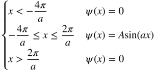
1.5 The wavefunction of an electron in one dimension is given as follows:
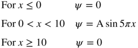
- Normalise the wavefunction by determining the value of A.
- What is the probability of finding the electron in the range 3 ≤ x ≤ 4?
- What is the probability of finding the electron in the range 3 ≤ x ≤ 3.1?
- Make a plot of |ψ|2 as a function of x.
-
1.6 The solution of Example 1.9 may be simplified in the limiting case in which Φ = ∞.
- Starting from Eq. 1.16, show that the allowed energy values in this limiting case are
where n is a quantum number. Hint: The wave functions must be zero outside the well. Also the boundary condition that

 is continuous is no longer relevant since the Schrödinger equation now includes an infinite value of Φ.
 - Determine the symmetric and anti‐symmetric wavefunctions.
- Is there a restriction on the values of quantum number n ?
- Plot the first five wavefunctions starting from the ground state as a function of x .
- Plot |ψ|2 as a function of x for each of the five wavefunctions of (d).
- Starting from Eq. 1.16, show that the allowed energy values in this limiting case are
-
1.7 Find the expected value of position and the expected value of momentum for the following wavefunctions:
-
- ψ(x) = Aexp(ikx)
-
- 1.8 Normalise the wavefunctions that are solutions to the problem in Example 1.9.
-
1.9 Owing to a supply of extra available energy we find that an electron in the potential well of Example 1.9 is equally likely to be found in all five of the lowest energy levels that are solutions to the Schrödinger equation rather than being in the ground state in the absence of this extra energy.
Since this electron is in any one of five quantum states ψ n that are each solutions to the Schrödinger equation we call this a superposition state ψ s , which is written as:

Note that the superposition state will also be a valid solution to the Schrödinger equation since the equation is a linear differential equation.
- Find the expected value of the energy of this electron. Neglect spin.
- Using a spreadsheet program such as Excel, Plot |ψ s(x)|2 along the x‐axis.
- What does the result of (b) tell you about the probability of finding the electron as a function of position along the x‐axis?
- The well of Example 1.9 is altered to have infinitely high walls such that it has more than five solutions to the Schrödinger equation. If the number of solutions is n and 5 < n < ∞, discuss how the result of part (b) might evolve as n approaches infinity.
- 1.10 The concept of observable electron spin magnetic moment having only two possible orientations, namely spin up and spin down, is difficult to accept because we rightly expect that the silver atoms in the type of experiment performed by Stern and Gerlach are randomly oriented when they emerge from the furnace. Do an Internet search and read discussions of how physicists attempt to rationalise our inability to explain how all but two of these orientations ‘disappear’. Write a two page summary of your findings.
- 1.11 The hydrogen atom contains one electron that exists in the potential V(r, θ, φ) caused by a positively charged nucleus. The Schrödinger equation can be solved for the electron wavefunctions and eigenenergies for the hydrogen atom provided we use spherical polar coordinates rather than Cartesian coordinates. Find a suitable textbook on atomic quantum mechanics (see, for example, Further Reading) that contain the solution to this problem and summarise the method and the results in 3–4 pages.
-
1.12 Find the solutions to the Schrödinger equation for the one‐dimensional double potential well shown below if
 and Φ = 5 eV. This type of double well can be used to model two adjacent atoms in a semiconductor crystal, and a similar model will be extended to an infinite number of atoms in Chapter 2.
- Find the possible values of electron energy E and sketch the wavefunctions of all solutions for which Φ − E > 0.
- Plot |ψ|2 as a function of x for each possible wavefunction.
What is the significance of the finite chance finding of the electron in the region
 ?
?