
![]()
Table Structures and Indexing
A lot of us have jobs where we need to give people structure but that is different from controlling.
—Keith Miller
To me, the true beauty of the relational database engine comes from its declarative nature. As a programmer, I simply ask the engine a question, and it answers it. The questions I ask are usually pretty simple; just give me some data from a few tables, correlate it on some of the data, do a little math perhaps, and give me back these pieces of information (and naturally do it incredibly fast if you don’t mind). Generally, the engine obliges with an answer extremely quickly. But how does it do it? If you thought it was magic, you would not be right. It is a lot of complex code implementing a massive amount of extremely complex algorithms that allow the engine to answer your questions in a timely manner. With every passing version of SQL Server, that code gets better at turning your relational request into a set of operations that gives you the answers you desire in remarkably small amounts of time. These operations will be shown to you on a query plan, which is a blueprint of the algorithms used to execute your query. I will use query plans often in this chapter and others to show you how your design choices can affect the way work gets done.
Our job as data-oriented designers and programmers is to assist the query optimizer (which takes your query and turns it into a plan of how to run the query), the query processor (which takes the plan and uses it to do the actual work), and the storage engine (which manages IO for the whole process) by first designing and implementing as close to the relational model as possible by normalizing your structures, using good set-based code (no cursors), following best practices with coding T-SQL, and so on. This is a design book, so I won’t cover T-SQL coding, but it is a skill you should master. Consider Apress’s Beginning T-SQL 2012 by Kathi Kellenberger (Aunt Kathi!) and Scott Shaw or perhaps one of Itzik Ben-Gan’s Inside SQL books on T-SQL for some deep learning on the subject. Once you have built your system correctly, the next step is to help out by adjusting the physical structures using indexing, filegroups, files, partitioning, and everything else you can do to adjust the physical layers to assist the optimizer deal with your commonly asked questions.
When it comes to tuning your database structures, you must maintain a balance between doing too much and too little. Indexing strategies are a great example of this. If you don’t use indexes enough, searches will be slow, as the query processor could have to read every row of every table for every query (which, even if it seems fast on your machine, can cause the concurrency issues we will cover in the next chapter by forcing the query processor to lock a lot more resources than is necessary). Use too many indexes, and modifying data could take too long, as indexes have to be maintained. Balance is the key, kind of like matching the amount of fluid to the size of the glass so that you will never have to answer that annoying question about a glass that has half as much fluid as it can hold. (The answer is either that the glass is too large or the waitress needs to refill your glass immediately, depending on the situation.)
Everything we have done so far has been centered on the idea that the quality of the data is the number one concern. Although this is still true, in this chapter, we are going to assume that we’ve done our job in the logical and implementation phases, so the data quality is covered. Slow and right is always better than fast and wrong (how would you like to get paid a week early, but only get half your money?), but the obvious goal of building a computer system is to do things right and fast. Everything we do for performance should affect only the performance of the system, not the data quality in any way.
We have technically added indexes in previous chapters as a side effect of adding primary key and unique constraints (in that a unique index is built by SQL Server to implement the uniqueness condition). In many cases, those indexes will turn out to be a lot of what you need to make normal queries run nicely, since the most common searches that people will do will be on identifying information. Of course, you will likely discover that some of the operations you are trying to achieve won’t be nearly as fast as you hope. This is where physical tuning comes in, and at this point, you need to understand how tables are structured and consider organizing the physical structures.
The goal of this chapter is to provide a basic understanding of the types of things you can do with the physical database implementation, including the indexes that are available to you, how they work, and how to use them in an effective physical database strategy. This understanding relies on a base knowledge of the physical data structures on which we based these indexes—in other words, of how the data is structured in the physical SQL Server storage engine. In this chapter, I’ll cover the following:
- Physical database structure: An overview of how the database and tables are stored. This acts mainly as foundation material for subsequent indexing discussion, but the discussion also highlights the importance of choosing and sizing your datatypes carefully.
- Indexing: A survey of the different types of indexes and their structure. I’ll demonstrate many of the index settings and how these might be useful when developing your strategy, to correct any performance problems identified during optimization testing.
- Index usage scenarios: I’ll discuss a few specialized cases of how to apply and use indexes.
- Index Dynamic Management View queries: In this section, I will introduce a couple of the dynamic management views that you can use to help determine what indexes you may need and to see which indexes have been useful in your system.
Once you understand the physical data structures, it will be a good bit easier to visualize what is occurring in the engine and then optimize data storage and access without affecting the correctness of the data. It’s essential to the goals of database design and implementation that the physical storage not affect the physically implemented model. This is what Codd’s eighth rule, also known as the Physical Data Independence rule—is about. As we discussed in Chapter 1, this rule states that the physical storage can be implemented in any manner as long as the users don’t have to know about it. It also implies that if you change the physical storage, the users shouldn’t be affected. The strategies we will cover should change the physical model but not the model that the users (people and code) know about. All we want to do is enhance performance, and understanding the way SQL Server stores data is an important step.
![]() Note I am generally happy to treat a lot of the deeper internals of SQL Server as a mystery left to the engine to deal with. For a deeper explanation consider any of Kalen Delaney’s books, where I go whenever I feel the pressing need to figure out why something that seems bizarre is occurring. The purpose of this chapter is to give you a basic feeling for what the structures are like, so you can visualize the solution to some problems and understand the basics of how to lay out your physical structures.
Note I am generally happy to treat a lot of the deeper internals of SQL Server as a mystery left to the engine to deal with. For a deeper explanation consider any of Kalen Delaney’s books, where I go whenever I feel the pressing need to figure out why something that seems bizarre is occurring. The purpose of this chapter is to give you a basic feeling for what the structures are like, so you can visualize the solution to some problems and understand the basics of how to lay out your physical structures.
Some of the samples may not work 100% the same way on your computer, depending on our hardware situations, or changes to the optimizer from updates or service packs.
Physical Database Structure
In SQL Server, databases are physically structured as several layers of containers that allow you to move parts of the data around to different disk drives for optimum access. As discussed in Chapter 1, a database is a collection of related data. At the logical level, it contains tables that have columns that contain data. At the physical level, databases are made up of files, where the data is physically stored. These files are basically just typical Microsoft Windows files, and they are logically grouped into filegroups that control where they are stored on a disk. Each file contains a number of extents, which are is an allocation of 64-KB in a database file that’s made up of eight individual contiguous 8-KB pages. The page is the basic unit of data storage in SQL Server databases. Everything that’s stored in SQL Server is stored on pages of several types—data, index, overflow and others—but these are the ones that are most important to you (I will list the others later in the section called “Extents and Pages”). The following sections describe each of these containers in more detail, so you understand the basics of how data is laid out on disk.
![]() Note Because of the extreme variety of hardware possibilities and needs, it’s impossible in a book on design to go into serious depth about how and where to place all your files in physical storage. I’ll leave this task to the DBA-oriented books. For detailed information about choosing and setting up your hardware, check out
http://msdn.microsoft.com
or most any of Glenn Berry’s writing. Glenn’s blog (at
http://sqlserverperformance.wordpress.com/
at the time of this writing) contained a wealth of information about SQL Server hardware, particularly CPU changes.
Note Because of the extreme variety of hardware possibilities and needs, it’s impossible in a book on design to go into serious depth about how and where to place all your files in physical storage. I’ll leave this task to the DBA-oriented books. For detailed information about choosing and setting up your hardware, check out
http://msdn.microsoft.com
or most any of Glenn Berry’s writing. Glenn’s blog (at
http://sqlserverperformance.wordpress.com/
at the time of this writing) contained a wealth of information about SQL Server hardware, particularly CPU changes.
Figure 10-1 provides a high-level depiction of the objects used to organize the files (I’m ignoring logs in this chapter, because you don’t have direct access to them).
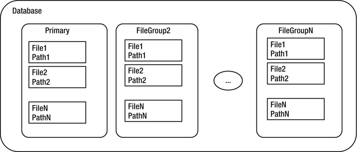
Figure 10-1. Database storage organization
At the top level of a SQL Server instance, we have the database. The database is comprised of one or more filegroups, which are logical groupings of one or more files. We can place different filegroups on different disk drives (hopefully on a different disk drive controller) to distribute the I/O load evenly across the available hardware. It’s possible to have multiple files in the filegroup, in which case SQL Server allocates space across each file in the filegroup. For best performance, it’s generally best to have no more files in a filegroup than you have physical CPUs (not including hyperthreading, though the rules with hyperthreading are changing as processors continue to improve faster than one could write books on the subject).
A filegroup contains one or more files, which are actual operating system files. Each database has at least one primary filegroup, whose files are called primary files (commonly suffixed as .mdf, although there’s no requirement to give the files any particular names or extension). Each database can possibly have other secondary filegroups containing the secondary files (commonly suffixed as .ndf), which are in any other filegroups. Files may only be a part of a single filegroup. SQL Server proportionally fills files by allocating extents in each filegroup equally, so you should make all of the files the same size if possible. (There is also a file type for full-text indexing and a filegroup type we used in Chapter 7 for filestream types of data that I will largely ignore in this chapter as well. I will focus only on the core file types that you will use for implementing your structures.)
You control the placement of objects that store physical data pages at the filegroup level (code and metadata is always stored on the primary filegroup, along with all the system objects). New objects created are placed in the default filegroup, which is the PRIMARY filegroup (every database has one as part of the CREATE DATABASE statement, or the first file specified is set to primary) unless another filegroup is specified in any CREATE <object> commands. For example, to place an object in a filegroup other than the default, you need to specify the name of the filegroup using the ON clause of the table- or index-creation statement:
CREATE TABLE <tableName>
(…) ON <fileGroupName>
This command assigns the table to the filegroup, but not to any particular file. Where in the files the object is created is strictly out of your control.
![]() Tip If you want to move a table to a different filegroup, you can use the MOVE TO option of the ALTER TABLE statement if the table has a clustered index, or for a heap (a table without a clustered index, covered later in this chapter), create a clustered index on the object on the filegroup you want it and then drop it. For nonclustered indexes, use the DROP_EXISTING setting on the CREATE INDEX statement.
Tip If you want to move a table to a different filegroup, you can use the MOVE TO option of the ALTER TABLE statement if the table has a clustered index, or for a heap (a table without a clustered index, covered later in this chapter), create a clustered index on the object on the filegroup you want it and then drop it. For nonclustered indexes, use the DROP_EXISTING setting on the CREATE INDEX statement.
Use code like the following to create indexes and specify a filegroup:
CREATE INDEX <indexName> ON <tableName> (<columnList>) ON <filegroup>;
Use the following type of command (or use ALTER TABLE) to create constraints that in turn create indexes (UNIQUE, PRIMARY KEY):
CREATE TABLE <tableName>
(
…
<primaryKeyColumn> int CONSTRAINT PKTableName ON <fileGroup>
…
);
For the most part, having just one filegroup and one file is the best practice for a large number of databases. If you are unsure if you need multiple filegroups, my advice is to build your database on a single filegroup and see if the data channel provided can handle the I/O volume (for the most part, I will avoid making too many such generalizations, as tuning is very much an art that requires knowledge of the actual load the server will be under). As activity increases and you build better hardware with multiple CPUs and multiple drive channels, you might place indexes on their own filegroup, or even place files of the same filegroup across different controllers.
In the following example, I create a sample database with two filegroups, with the secondary filegroup having two files in it (I put this sample database in an SQLData folder in the root of the C drive to keep the example simple (and able to work on the types of drives that many of you will probably be testing my code on), but it is rarely a good practice to place your files on the C: drive when you have others available. I generally put a sql directory on every drive and put everything SQL in that directory in subfolders to keep things consistent over all of our servers. Put the files wherever works best for you.):
CREATE DATABASE demonstrateFilegroups ON
PRIMARY ( NAME = Primary1, FILENAME = 'c:sqldatademonstrateFilegroups_primary.mdf',
SIZE = 10MB),
FILEGROUP SECONDARY
( NAME = Secondary1, FILENAME = 'c:sqldatademonstrateFilegroups_secondary1.ndf',
SIZE = 10MB),
( NAME = Secondary2, FILENAME = 'c:sqldatademonstrateFilegroups_secondary2.ndf',
SIZE = 10MB)
LOG ON ( NAME = Log1,FILENAME = 'c:sqllogdemonstrateFilegroups_log.ldf', SIZE = 10MB);
You can define other file settings, such as minimum and maximum sizes and growth. The values you assign depend on what hardware you have. For growth, you can set a FILEGROWTH parameter that allows you to grow the file by a certain size or percentage of the current size, and a MAXSIZE parameter, so the file cannot just fill up existing disk space. For example, if you wanted the file to start at 1GB and grow in chunks of 100MB up to 2GB, you could specify the following:
CREATE DATABASE demonstrateFileGrowth ON
PRIMARY ( NAME = Primary1,FILENAME = 'c:sqldatademonstrateFileGrowth_primary.mdf',
SIZE = 1GB, FILEGROWTH=100MB, MAXSIZE=2GB)
LOG ON ( NAME = Log1,FILENAME = 'c:sqlldatademonstrateFileGrowth_log.ldf', SIZE = 10MB);
The growth settings are fine for smaller systems, but it’s usually better to make the files large enough so that there’s no need for them to grow. File growth can be slow and cause ugly bottlenecks when OLTP traffic is trying to use a file that’s growing. When SQL Server is running on a desktop operating system like Windows XP or greater (and at this point you probably ought to be using something greater like Windows 7—(or presumably Windows 8 or 9 depending on when you are reading this) or on a server operating system such as Windows Server 2003 or greater (again, it is 2012, so emphasize “or greater”), you can improve things by using “instant” file allocation (though only for data files). Instead of initializing the files, the space on disk can simply be allocated and not written to immediately. To use this capability, the system account cannot be LocalSystem, and the user account that the SQL Server runs under must have SE_MANAGE_VOLUME_NAME Windows permissions. Even with the existence of instant file allocation, it’s still going to be better to have some idea of what size data you will have and allocate space proactively, as you then have cordoned off the space ahead of time: no one else can take it from you, and you won’t fail when the file tries to grow and there isn’t enough space. In either event, the DBA staff should be on top of the situation and make sure that you don’t run out of space.
You can query the sys.filegroups catalog view to view the files in the newly created database:
USE demonstrateFilegroups;
GO
SELECT case WHEN fg.name IS NULL
then CONCAT('OTHER-',df.type_desc COLLATE database_default)
ELSE fg.name end as file_group,
df.name as file_logical_name,
df.physical_name as physical_file_name
FROM sys.filegroups fg
RIGHT JOIN sys.database_files df
ON fg.data_space_id = df.data_space_id;
This returns the following results:
| file_group | file_logical_name | physical_file_name |
| ========= | ------------- | ------------- |
| PRIMARY | Primary1 | c:sqldatademonstrateFilegroups_primary.mdf |
| OTHER-LOG | Log1 | c:sqllogdemonstrateFilegroups_log.ldf |
| SECONDARY | Secondary1 | c:sqldatademonstrateFilegroups_secondary1.ndf |
| SECONDARY | Secondary2 | c:sqldatademonstrateFilegroups_secondary2.ndf |
The LOG file isn’t technically part of a filegroup, so I used a right outer join to the database files and gave it a default filegroup name of OTHER plus the type of file to make the results include all files in the database. You may also notice a couple other interesting things in the code. First, the CONCAT function is new to SQL Server 2012 to add strings together.. Second is the COLLATE database_default. The strings in the system functions are in the collation of the server, while the literal OTHER- is in the database collation. If the server doesn’t match the database, this query would fail.
There’s a lot more information than just names in the catalog views I’ve referenced already in this chapter. If you are new to the catalog views, dig in and learn them. There is a wealth of information in those views that will be invaluable to you when looking at systems to see how they are set up and to determine how to tune them.
![]() Tip An interesting feature of filegroups is that you can back up and restore them individually. If you need to restore and back up a single table for any reason, placing it in its own filegroup can achieve this.
Tip An interesting feature of filegroups is that you can back up and restore them individually. If you need to restore and back up a single table for any reason, placing it in its own filegroup can achieve this.
These databases won’t be used anymore, so if you created them, just drop them if you desire:
USE MASTER;
GO
DROP DATABASE demonstrateFileGroups;
GO
DROP DATABASE demonstrateFileGrowth;
Extents and Pages
As shown in Figure 10-2, files are further broken down into a number of extents , each consisting of eight separate 8-KB pages where tables, indexes, and so on are physically stored. SQL Server only allocates space in a database to extents. When files grow, you will notice that the size of files will be incremented only in 64-KB increments.
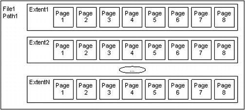
Figure 10-2. Files and extents
Each extent in turn has eight pages that hold one specific type of data each:
- Data: Table data.
- Index: Index data.
- Overflow data : Used when a row is greater than 8,060 bytes or for varchar(max), varbinary(max), text, or image values.
- Allocation map : Information about the allocation of extents.
- Page free space : Information about what different pages are allocated for.
- Index allocation : Information about extents used for table or index data.
- Bulk changed map : Extents modified by a bulk INSERT operation.
- Differential changed map : Extents that have changed since the last database backup command. This is used to support differential backups.
In larger databases, most extents will contain just one type of page, but in smaller databases, SQL Server can place any kind of page in the same extent. When all data is of the same type, it’s known as a uniform extent. When pages are of various types, it’s referred to as a mixed extent.
SQL Server places all table data in pages, with a header that contains metadata about the page (object ID of the owner, type of page, and so on), as well as the rows of data, which I’ll cover later in this chapter. At the end of the page are the offset values that tell the relational engine where the rows start.
Figure 10-3 shows a typical data page from a table. The header of the page contains identification values such as the page number, the object ID of the object the data is for, compression information, and so on. The data rows hold the actual data. Finally, there’s an allocation block that has the offsets/pointers to the row data.
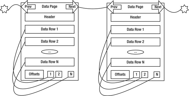
Figure 10-3. Data pages
Figure 10-3 shows that there are pointers from the next to the previous rows. These pointers are only used when pages are ordered, such as in the pages of an index. Heap objects (tables with no clustered index) are not ordered. I will cover this a bit later in the “Index Types” section.
The other kind of page that is frequently used that you need to understand is the overflow page . It is used to hold row data that won’t fit on the basic 8,060-byte page. There are two reasons an overflow page is used:
- The combined length of all data in a row grows beyond 8,060 bytes. In versions of SQL Server prior to 2000, this would cause an error. In versions after this, data goes on an overflow page automatically, allowing you to have virtually unlimited row sizes.
- By setting the sp_tableoption setting on a table for large value types out of row to 1, all the (max) and XML datatype values are immediately stored out of row on an overflow page. If you set it to 0, SQL Server tries to place all data on the main page in the row structure, as long as it fits into the 8,060-byte row. The default is 0, because this is typically the best setting when the typical values are short enough to fit on a single page.
For example, Figure 10-4 depicts the type of situation that might occur for a table that has the large value types out of row set to 1. Here, Data Row 1 has two pointers to a varbinary(max) columns: one that spans two pages and another that spans only a single page. Using all of the data in Data Row 1 will now require up to four reads (depending on where the actual page gets stored in the physical structures), making data access far slower than if all of the data were on a single page. This kind of performance problem can be easy to overlook, but on occasion, overflow pages will really drag down your performance, especially when other programmers use SELECT * on tables where they don’t really need all of the data.
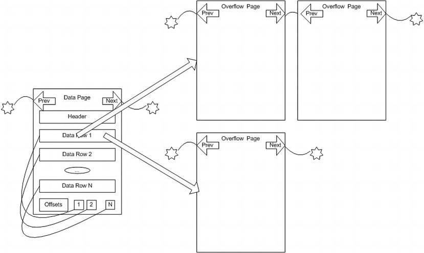
Figure 10-4. Sample overflow pages
The overflow pages are linked lists that can accommodate up to 2GB of storage in a single column. Generally speaking, it isn’t really a very good idea to store 2GB in a single column (or even a row), but the ability to do so is available if needed.
Understand that storing large values that are placed off of the main page will be far more costly when you need these values than if all of the data can be placed in the same data page. On the other hand, if you seldom use the data in your queries, placing them off the page can give you a much smaller footprint for the important data, requiring far less disk access on average. It is a balance that you need to take care with, as you can imagine how costly a table scan of columns that are on the overflow pages is going to be. Not only will you have to read extra pages, you have to be redirected to the overflow page for every row that’s overflowed.
Be careful when allowing data to overflow the page. It’s guaranteed to make your processing more costly, especially if you include the data that’s stored on the overflow page in your queries—for example, if you use the dreaded SELECT * regularly in production code! It’s important to choose your datatypes correctly to minimize the size of the data row to include only frequently needed values. If you frequently need a large value, keep it in row; otherwise, consider placing it off row or even create two tables and join them together as needed.
![]() Tip The need to access overflow pages is just one of the reasons to avoid using SELECT * FROM <tablename>–type queries in your production code, but it is an important one. Too often, you get data that you don’t intend to use, and when that data is located off the main data page, performance could suffer tremendously, and, in most cases, needlessly.
Tip The need to access overflow pages is just one of the reasons to avoid using SELECT * FROM <tablename>–type queries in your production code, but it is an important one. Too often, you get data that you don’t intend to use, and when that data is located off the main data page, performance could suffer tremendously, and, in most cases, needlessly.
Data on Pages
When you get down to the row level, the data is laid out with metadata, fixed length fields, and variable length fields, as shown in Figure 10-5. (Note that this is a generalization, and the storage engine does a lot of stuff to the data for optimization, especially when you enable compression.)

Figure 10-5. Data row
The metadata describes the row, gives information about the variable length fields, and so on. Generally speaking, since data is dealt with by the query processor at the page level, even if only a single row is needed, data can be accessed very rapidly no matter the exact physical representation.
![]() Note I use the term “column” when discussing logical SQL objects such as tables and indexes, but when discussing the physical table implementation, “field” is the proper term. Remember from Chapter 1 that a field is a physical location within a record.
Note I use the term “column” when discussing logical SQL objects such as tables and indexes, but when discussing the physical table implementation, “field” is the proper term. Remember from Chapter 1 that a field is a physical location within a record.
The maximum amount of data that can be placed on a single page (including overhead from variable fields) is 8,060 bytes. As illustrated in Figure 10-4, when a data row grows larger than 8,060 bytes, the data in variable length columns was can spill out onto an overflow page. A 16-byte pointer is left on the original page and points to the page where the overflow data is placed.
When inserting or updating rows, SQL Server might have to rearrange the data on the pages due to the pages being filled up. Such rearranging can be a particularly costly operation. Consider the situation from our example shown in Figure 10-6, assuming that only three values can fit on a page.
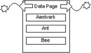
Figure 10-6. Sample data page before page split
Say we want to add the value Bear to the page. If that value won’t fit onto the page, the page will need to be reorganized. Pages that need to be split are split into two, generally with 50 percent of the data on one page, and 50 percent on the other (there are usually more than three values on a real page). Once the page is split and its values are reinserted, the new pages would end up looking something like Figure 10-7.
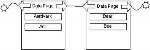
Figure 10-7. Sample data page after page split
Page splits are awfully costly operations and can be terrible for performance, because after the page split, data won’t be located on successive physical pages. This condition is commonly known as fragmentation. Page splits occur in a normal system and are simply a part of adding data to your table. However, they can occur extremely rapidly and seriously degrade performance if you are not careful. Understanding the effect that page splits can have on your data and indexes is important as you tune performance on tables that have large numbers of inserts or updates.
To tune your tables and indexes to help minimize page splits, you can use the FILL FACTOR of the index. When you build or rebuild an index or a table (using ALTER TABLE <tablename> REBUILD, a command that was new in SQL Server 2008), the fill factor indicates how much space is left on each page for future data. If you are inserting random values all over the structures, a common situation that occurs when you use a nonsequential uniqueidentifier for a primary key, you will want to leave adequate space on each page to cover the expected numbers of rows that will be created in the future. During a page split, the data page is always split approximately fifty-fifty, and it is left half empty on each page, and even worse, the structure is becoming, as mentioned, fragmented.
Let’s jump ahead a bit: one of the good things about using a monotonously increasing value for a clustered index is that page splits over the entire index are greatly decreased. The table grows only on one end of the index, and while the index does need to be rebuilt occasionally using ALTER INDEX REORGANIZE or ALTER INDEX REBUILD, you don’t end up with page splits all over the table. And since the new value that won’t fit on the page comes at the end of the table, instead of a split, another page can be added to the chain. In the “Index Dynamic Management Views” section later, I will provide a query that will help you to know when to rebuild the index due to fragmentation.
Compression
The reason that the formats for pages and rows are generalized in the previous sections is that in SQL Server 2008, Microsoft implemented compression of data at the row and page levels. In versions prior to SQL Server 2005 SP2, all data was stored on a page in a raw format. However, in SQL Server 2005 SP2, Microsoft introduced datatype-level compression, which allowed data of the decimal datatype to be stored in a variable length field, also referred to as vardecimal. For SQL Server 2005, datatype compression was set using the sp_tableoption procedure with a setting of 'vardecimal storage format'.
In SQL Server 2008, the concept of compression was extended even further to all of the fixed length datatypes, including int, char, and float. Basically, you can allow SQL Server to save space by storing your data like it was a variable-sized type, yet in usage, the data will appear and behave like a fixed length type. Then in 2008R2, the feature was expanded yet again to include Unicode values. In Appendix A, I will note how compression will affect each datatype individually.
For example, if you stored the value of 100 in an int column, SQL Server needn’t use all 32 bits; it can store the value 100 the same amount of space as a tinyint. So instead of taking a full 32 bits, SQL Server can simply use 8 bits (1 byte). Another case is when you use a fixed length type like char(30) column but store only two characters; 28 characters could be saved, and the data padded as it is used. There is an overhead of 2 bytes per variable length column (or 4 bits if the size of the column is less than 8 bytes). Note that compression is only available in the Enterprise Edition.
This datatype-level compression is referred to as row compression , where each row in the table will be compressed as datatypes allow, shrinking the size on disk, but not making any major changes to the page structure. In Appendix B, I will indicate how each of the datatypes is affected by row compression, or for a list that may show any recent changes, you can check SQL Server Books Online for the topic of “Row Compression Implementation.” Row compression is a very interesting thing for many databases that use lots of fixed length data (for example, integers, especially for surrogate keys).
SQL Server also includes an additional compression capability called page compression. With page compression, first the data is compressed in the same manner as row compression, and then, the storage engine does a couple of interesting things to compress the data on a page:
- Prefix compression : Looks for repeated values in a value (like '0000001' and compresses the prefix to something like 6-0 (six zeros)
- Dictionary compression : For all values on the page, the storage engine looks for duplication, stores the duplicated value once, and then stores pointers on the data pages where the duplicated values originally resided.
You can apply data compression to your tables and indexes with the CREATE TABLE, ALTER TABLE, CREATE INDEX, and ALTER INDEX syntaxes. As an example, I will create a simple table, called test, and enable page compression on the table, row compression on a clustered index, and page compression on another index. (This code will work only on an Enterprise installation, or if you are using Developer Edition for testing.)
USE tempdb;
GO
CREATE TABLE testCompression
(
testCompressionId int NOT NULL,
value int NOT NULL
);
WITH (DATA_COMPRESSION = ROW) -- PAGE or NONE
ALTER TABLE testCompression REBUILD WITH (DATA_COMPRESSION = PAGE);
CREATE CLUSTERED INDEX XTestCompression_value
ON testCompression (value) WITH ( DATA_COMPRESSION = ROW );
ALTER INDEX XTestCompression_value
ON testCompression REBUILD WITH ( DATA_COMPRESSION = PAGE );
![]() Note The syntax of the
CREATE INDEX command allows for compression of the partitions of an index in different manners. I mention partitioning in the next section of the chapter. For full syntax, refer to SQL Server Books Online.
Note The syntax of the
CREATE INDEX command allows for compression of the partitions of an index in different manners. I mention partitioning in the next section of the chapter. For full syntax, refer to SQL Server Books Online.
Giving advice on whether to use compression is not really possible without knowing the factors that surround your actual situation. One tool you should use is the system procedure—sp_estimate_data_compression_savings—to check existing data to see just how compressed the data in the table or index would be after applying compression, but it won’t tell you how the compression will positively or negatively affect your performance. There are trade-offs to any sorts of compression. CPU utilization will go up in most cases, because instead of directly using the data right from the page, the query processor will have to translate the values from the compressed format into the uncompressed format that SQL Server will use. On the other hand, if you have a lot of data that would benefit from compression, you could possibly lower your I/O enough to make doing so worth the cost. Frankly, with CPU power growing by leaps and bounds with multiple-core scenarios these days and I/O still the most difficult to tune, compression could definitely be a great thing for many systems. However, I suggest testing with and without compression before applying in your production systems.
The last general physical structure concept that I will introduce is partitioning. Partitioning allows you to break a table (or index) into multiple physical structures by breaking them into more manageable chunks. Partitioning can allow SQL Server to scan data from different processes, enhancing opportunities for parallelism. SQL Server 7.0 and 2000 had partitioned views, where you would define a view and a set of tables, with each serving as a partition of the data. If you have properly defined (and trusted) constraints, SQL Server would use the WHERE clause to know which of the tables referenced in the view would have to be scanned in response to a given query. The data in the view was also editable like in a normal table. One thing you still can do with partitioned views is to build distributed partitioned views, which reference tables on different servers.
In SQL Server 2005, you could begin to define partitioning as part of the table structure. Instead of making a physical table for each partition, you define, at the DDL level, the different partitions of the table. Internally, the table is broken into the partitions based on a scheme that you set up. Note, too, that this feature is only included in the Enterprise Edition.
At query time, SQL Server can then dynamically scan only the partitions that need to be searched, based on the criteria in the WHERE clause of the query being executed. I am not going to describe partitioning too much, but I felt that it needed a mention in this edition of this book as a tool at your disposal with which to tune your databases, particularly if they are very large or very active. For deeper coverage, I would suggest you consider on of Kalen Delaney’s SQL Server Internals books. They are the gold standard in understanding the internals of SQL Server.
I will, however, present the following basic example of partitioning. Use whatever database you desire. I used tempdb for the data and AdventureWorks2012 for the sample data on my test machine and included the USE statement in the code download. The example is that of a sales order table. I will partition the sales into three regions based on the order date. One region is for sales before 2006, another for sales between 2006 and 2007, and the last for 2007 and later. The first step is to create a partitioning function. You must base the function on a list of values, where the VALUES clause sets up partitions that the rows will fall into based on the smalldatetime values that are presented to it, for example:
CREATE PARTITION FUNCTION PartitionFunction$dates (smalldatetime)
AS RANGE LEFT FOR VALUES ('20060101','20070101'),
--set based on recent version of
--AdventureWorks2012.Sales.SalesOrderHeader table to show
--partition utilization
Specifying the function as RANGE LEFT says that the values in the comma-delimited list should be considered the boundary on the side listed. So in this case, the ranges would be as follows:
- value <= '20060101'
- value > '20060101' and value <= '20070101'
- value > '20070101'
Specifying the function as RANGE RIGHT would have meant that the values lie to the right of the values listed, in the case of our ranges, for example:
- value < '20060101'
- value >= '20060101' and value < '20070101'
- value >= '20070101'
Next, use that partition function to create a partitioning scheme:
CREATE PARTITION SCHEME PartitonScheme$dates
AS PARTITION PartitionFunction$dates ALL to ( [PRIMARY] );
which will let you know:
Partition scheme 'PartitonScheme$dates' has been created successfully. 'PRIMARY' is marked as the next used filegroup in partition scheme 'PartitonScheme$dates'.
With the CREATE PARTITION SCHEME command, you can place each of the partitions you previously defined on a specific filegroup. I placed them all on the same filegroup for clarity and ease, but in practice, you usually want them on different filegroups, depending on the purpose of the partitioning. For example, if you were partitioning just to keep the often-active data in a smaller structure, placing all partitions on the same filegroup might be fine. But if you want to improve parallelism or be able to just back up one partition with a filegroup backup, you would want to place your partitions on different filegroups.
Next, you can apply the partitioning to a new table. You’ll need a clustered index involving the partition key. You apply the partitioning to that index. Following is the statement to create the partitioned table:
CREATE TABLE dbo.salesOrder
(
salesOrderIdint NOT NULL,
customerIdint NOT NULL,
orderAmountdecimal(10,2) NOT NULL,
orderDatesmalldatetime NOT NULL,
CONSTRAINT PKsalesOrder primary key nonclustered (salesOrderId)
ON [Primary],
CONSTRAINT AKsalesOrder unique clustered (salesOrderId, orderDate)
) on PartitonScheme$dates (orderDate);
Next, load some data from the AdventureWorks2012.Sales.SalesOrderHeader table to make looking at the metadata more interesting. You can do that using an INSERT statement such as the following:
INSERT INTO dbo.salesOrder(salesOrderId, customerId, orderAmount, orderDate)
SELECT SalesOrderID, CustomerID, TotalDue, OrderDate
FROM AdventureWorks2012.Sales.SalesOrderHeader;
You can see what partition each row falls in using the $partition function. You suffix the $partition function with the partition function name and the name of the partition key (or a partition value) to see what partition a row’s values are in, for example:
SELECT *, $partition.PartitionFunction$dates(orderDate) as partiton
FROM dbo.salesOrder;
You can also view the partitions that are set up through the sys.partitions catalog view. The following query displays the partitions for our newly created table:
SELECT partitions.partition_number, partitions.index_id,
partitions.rows, indexes.name, indexes.type_desc
FROM sys.partitions as partitions
JOIN sys.indexes as indexes
on indexes.object_id = partitions.object_id
AND indexes.index_id = partitions.index_id
WHERE partitions.object_id = object_id('dbo.salesOrder'),
This will return the following:
| partition_number | index_id | rows | name | type_desc |
| ========= | ------------- | ------------- | ------------- | ------------- |
| 1 | 1 | 1424 | 1424 | 1424 |
| 2 | 1 | 3720 | AKsalesOrder | CLUSTERED |
| 3 | 1 | 26321 | AKsalesOrder | CLUSTERED |
| 1 | 2 | 31465 | PKsalesOrder | NONCLUSTERED |
Partitioning is not a general purpose tool that should be used on every table, which is one of the reasons why it is only included in Enterprise Edition. However, partitioning can solve a good number of problems for you, if need be:
- Performance: If you only ever need the past month of data out of a table with three years’ worth of data, you can create partitions of the data where the current data is on a partition and the previous data is on a different partition.
- Rolling windows: You can remove data from the table by dropping a partition, so as time passes, you add partitions for new data and remove partitions for older data (or move to a different archive table).
- Maintainence: Some maintainance can be done at the partition level rather than the entire table, so once partition data is read-only, you may not need to maintain any longer. Some caveats do apply (you cannot rebuild a partitioned index online, for example.)
Indexes Overview
Indexes allow the SQL Server engine to perform fast, targeted data retrieval rather than simply scanning though the entire table. A well-placed index can speed up data retrieval by orders of magnitude, while a haphazard approach to indexing can actually have the opposite effect when creating, updating, or deleting data.
Indexing your data effectively requires a sound knowledge of how that data will change over time, the sort of questions that will be asked of it, and the volume of data that you expect to be dealing with. Unfortunately, this is what makes any topic about physical tuning so challenging. To index effectively, you almost need the psychic ability to fortell the future of your exact data usage patterns. Nothing in life is free, and the creation and maintenance of indexes can be costly. When deciding to (or not to) use an index to improve the performance of one query, you have to consider the effect on the overall performance of the system.
In the upcoming sections, I’ll do the following:
- Introduce the basic structure of an index.
- Discuss the two fundamental types of indexes and how their structure determines the structure of the table.
- Demonstrate basic index usage, introducing you to the basic syntax and usage of indexes.
- Show you how to determine whether SQL Server is likely to use your index and how to see if SQL Server has used your index.
If you are producing a product for sale that uses SQL Server as the backend, indexes are truly going to be something that you could let your customers manage unless you can truly effectively constrain how users will use your product. For example, if you sell a product that manages customers, and your basic expectation is that they will have around 1,000 customers, what happens if one wants to use it with 100,000 customers? Do you not take their money? Of course you do, but what about performance? Hardware improvements generally cannot even give linear improvement in performance. So if you get hardware that is 100 times “faster,” you would be extremely fortunate to get close to 100 times improvement. However, adding a simple index can provide 100,000 times improvement that may not even make a difference at all on the smaller data set. (This is not to pooh pooh the value of faster hardware at all. Just that situationally you get far greater gain from writing better code than you will from just throwing hardware at the problem. The ideal situation is adequate hardware and excellent code, naturally).
An index is an object that SQL Server can maintain to optimize access to the physical data in a table. You can build an index on one or more columns of a table. In essence, an index in SQL Server works on the same principle as the index of a book. It organizes the data from the column (or columns) of data in a manner that’s conducive to fast, efficient searching, so you can find a row or set of rows without looking at the entire table. It provides a means to jump quickly to a specific piece of data, rather than just starting on page one each time you search the table and scanning through until you find what you’re looking for. Even worse, unless SQL Server knows exactly how many rows it is looking for, it has no way to know if it can stop scanning data when one row had been found. Also, like the index of a book, an index is a separate entity from the actual table (or chapters) being indexed.
As an example, consider that you have a completely unordered list of employees and their details. If you had to search this list for persons named “Davidson”, you would have to look at every single name on every single page. Soon after trying this, you would immediately start trying to devise some better manner of searching. On first pass, you would probably sort the list alphabetically. But what happens if you needed to search for an employee by an employee identification number? Well, you would spend a bunch of time searching through the list sorted by last name for the employee number. Eventually, you could create a list of last names and the pages you could find them on and another list with the employee numbers and their pages. Following this pattern, you would build indexes for any other type of search you’d regularly perform on the list. Of course, SQL Server can page through the phone book one name at a time in such a manner that, if you need to do it occasionally, it isn’t such a bad thing, but looking at two or three names per search is always more efficient than two or three hundred, much less two or three million.
Now, consider this in terms of a table like an Employee table. You might execute a query such as the following:
SELECT LastName, <EmployeeDetails>
FROM Employee
WHERE LastName = 'Davidson';
In the absence of an index to rapidly search, SQL Server will perform a scan of the data in the entire table (referred to as a table scan) on the Employee table, looking for rows that satisfy the query predicate. A full table scan generally won’t cause you too many problems with small tables, but it can cause poor performance for large tables with many pages of data, much as it would if you had to manually look through 20 values versus 2,000. Of course, when you have a light load, like on your development box, you probably won’t be able to discern the difference between a seek and a scan (or even hundreds of scans). Only when you are experiencing a reasonably heavy load will the difference be noticed.
If we instead created an index on the LastName column, the index would sort the LastName rows in a logical fashion (in ascending alphabetical order by default) and the database engine can move directly to rows where the last name is Davidson and retrieve the required data quickly and efficiently. And even if there are ten people with the last name of Davidson, SQL Server knows to stop when it hits 'Davidtown'.
Of course, as you might imagine, the engineer types who invented the concept of indexing and searching data structures don’t simply make lists to search through. Instead, indexes are implemented using what is known as a balanced tree (B-tree) structure. The index is made up of index pages structured, again, much like an index of a book or a phone book. Each index page contains the first value in a range and a pointer to the next lower page in the index. The last level in the index is referred to as the leaf page, which contains the actual data values that are being indexed, plus either the data for the row or pointers to the data. This allows the query processor to go directly to the data it is searching for by checking only a few pages, even when there are a millions of values in the index.
Figure 10-8 shows an example of the type of B-tree that SQL Server uses for indexes. Each of the outer rectangles is an 8K index page, just as we discussed earlier. The three values—A, J, and P—are the index keys in this top-level page of the index. The index page has as many index keys as is possible. To decide which path to follow to reach the lower level of the index, we have to decide if the value requested is between two of the keys: A to I, J to P, or greater than P. For example, say the value we want to find in the index happens to be I. We go to the first page in the index. The database determines that I doesn’t come after J, so it follows the A pointer to the next index page. Here, it determines that I comes after C and G, so it follows the G pointer to the leaf page.
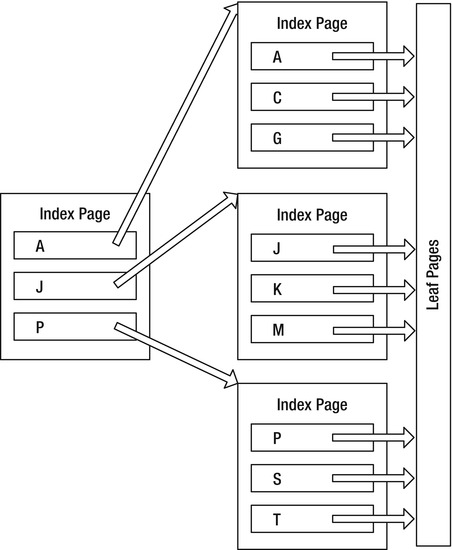
Figure 10-8. Basic index structure
Each of these pages is 8KB in size. Depending on the size of the key (determined by summing the data lengths of the columns in the key, up to a maximum of 900 bytes), it’s possible to have anywhere from 8 entries to over 1,000 on a single page. The more keys you can fit on a page, the greater the number of pages you can have on each level of the index. The more pages are linked from each level to the next, the fewer numbers of steps from the top page of the index to reach the leaf.
B-tree indexes are extremely efficient, because for an index that stores only 500 different values on a page—a reasonable number for a typical index of an integer—it has 500 pointers on the next level in the index, and the second level has 500 pages with 500 values each. That makes 250,000 different pointers on that level, and the next level has up to 250,000 * 500 pointers. That’s 125,000,000 different values in just a three-level index. Change that to a 100-byte key, do the math, and you will see why smaller keys are better! Obviously, there’s overhead to each index key, and this is just a rough estimation of the number of levels in the index.
Another idea that’s mentioned occasionally is how well balanced the tree is. If the tree is perfectly balanced, every index page would have exactly the same number of keys on it. Once the index has lots of data on one end, or data gets moved around on it for insertions or deletions, the tree becomes ragged, with one end having one level, and another many levels. This is why you have to do some basic maintenance on the indexes, something I have mentioned already.
Index Types
How indexes are structured internally is based on the existence (or nonexistence) of a clustered index. For the nonleaf pages of an index, everything is the same for all indexes. However, at the leaf node, the indexes get quite different—and the type of index used plays a large part in how the data in a table is physically organized.
There are two different types of relational indexes:
- Clustered: This type orders the physical table in the order of the index.
- Nonclustered: These are completely separate structures that simply speed access.
In the upcoming sections, I’ll discuss how the different types of indexes affect the table structure and which is best in which situation.
A clustered index physically orders the pages of the data in the table. The leaf pages of the clustered indexes are the data pages of the table. Each of the data pages is then linked to the next page in a doubly linked list to provide ordered scanning. The leaf pages of the clustered index are the actual data pages. In other words, the records in the physical structure are sorted according to the fields that correspond to the columns used in the index. Tables with clustered indexes are referred to as clustered tables.
The key of a clustered index is referred to as the clustering key, and this key will have additional uses that will be mentioned later in this chapter. For clustered indexes that aren’t defined as unique, each record has a 4-byte value (commonly known as an uniquifier) added to each value in the index where duplicate values exist. For example, if the values were A, B, and C, you would be fine. But, if you added another value B, the values internally would be A, B + 4ByteValue, B + Different4ByteValue, and C. Clearly, it is not optimal to get stuck with 4 bytes on top of the other value you are dealing with in every level of the index, so in general, you should try to use the clustered index on a set of columns where the values are unique.
Figure 10-9 shows, at a high level, what a clustered index might look like for a table of animal names. (Note that this is just a partial example, there would likely be more second-level pages for Horse and Python at a minimum.)
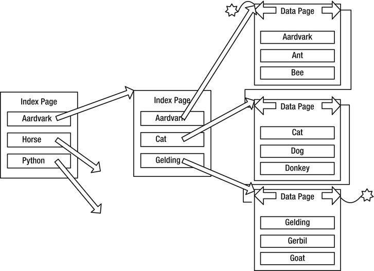
Figure 10-9. Clustered index example
You can have only one clustered index on a table, because the table cannot be ordered in more than one direction. (Remember this; it is one of the most fun interview questions. Answering anything other than “one clustered index per table” leads to a fun line of followup questioning.)
A good real-world example of a clustered index would be a set of old-fashioned encyclopedias. Each letter is a level of the index, and on each page, there is another level that denotes the things you can find on each page (e.g., Office–Officer). Then. each topic is the leaf level of the index. The encyclopedia is are clustered on the topics in these books, just as the example was clustered on the name of the animal. In essence, the entire book is a table of information in clustered ordered. And indexes can be partitioned as well. The encylopedias are partitioned by letter into multiple books.
Now, consider a dictionary. Why are the words sorted, rather than just having a separate index with the words not in order? I presume that at least part of the reason is to let the readers scan through words they don’t know exactly how to spell, checking the definition to see if the word matches what they expect. SQL Server does something like this when you do a search. For example, back in Figure 10-9, if you were looking for a cat named George, you could use the clustered index to find rows where animal = 'Cat', then scan the data pages for the matching pages for any rows where name = 'George'.
I must caution you that although it’s true, physically speaking, that tables are stored in the order of the clustered index; logically speaking, tables must be thought of as having no order. (I know I promised to not mention this again back in Chapter 1, but it really is an important thing to remember.) This lack of order is a fundamental truth of relational programming: you aren’t required to get back data in the same order when you run the same query twice. The ordering of the physical data can be used by the query processor to enhance your performance, but during intermediate processing, the data can be moved around in any manner that results in faster processing the answer to your query. It’s true that you do almost always get the same rows back in the same order, mostly because the optimizer is almost always going to put together the same plan every time the same query is executed under the same conditions. However, load up the server with many requests, and the order of the data might change so SQL Server can best use its resources, regardless of the data’s order in the structures. SQL Server can choose to return data to us in any order that’s fastest for it. If disk drives are busy in part of a table and it can fetch a different part, it will. If order matters, use an ORDER BY clause to make sure that data is returned as you want.
Nonclustered index structures are fully independent of the underlying table. Where a clustered index is like a dictionary with the index physically linked to the table (since the leaf pages of the index are a part of the table), nonclustered indexes are more like indexes in a textbook. A nonclustered index is completely separate from the data, and on the leaf page, there are pointers to go to the data pages much like the index of a book contains page numbers.
Each leaf page in a nonclustered index contains some form of pointer to the rows on the data page. The pointer from the index to a data row is known as a row locator. Exactly how the row locator of a nonclustered indexes is structured is based on whether or not the underlying table has a clustered index.
In this section, I will first show an abstract representation of the nonclustered index and then show the differences between the implementation of a nonclustered index when you do and do not also have a clustered index. At an abstract level, all nonclustered indexes follow the form shown in Figure 10-10.
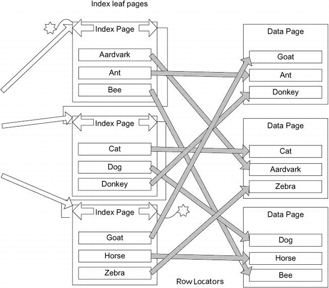
Figure 10-10. Sample nonclustered index
The major difference between the two possibilities comes down to the row locator being different based on whether the underlying table has a clustered index. There are two different types of pointer that will be used:
- Tables with a clustered index: Clustering key
- Tables without a clustered index: Pointer to physical location of the data
In the next two sections, I’ll explain these in more detail. New in 2012 is a new type of index that I will briefly mention called a columnstore index. Rather than store index data per row, they store data by column. They are typical indexes, in that they don’t change the structure of the data, but they do make the table read only. It is a very exciting feature for data warehouse types of queries, but in relational, OLTP databases, there isn’t really a use for columnstore indexes. In Chapter 14, a columnstore index will be used in an example for the data warehouse overview, but that will be the extent of discussion on the subject. They are structured quite differently from classic B-tree indices, so if you do get to building a data warehouse (or if you are also involved with building dimensional databases), you will want to understand how they work and how they are structured as they will likely provide your star schema queries with a tremendous performance increase.
![]() Tip You can place nonclustered indexes on a different filegroup than the data pages to maximize the use of your disk subsystem in parallel. Note that the filegroup you place the indexes on ought to be on a different controller channel than the table; otherwise, it’s likely that there will be minimal or no gain.
Tip You can place nonclustered indexes on a different filegroup than the data pages to maximize the use of your disk subsystem in parallel. Note that the filegroup you place the indexes on ought to be on a different controller channel than the table; otherwise, it’s likely that there will be minimal or no gain.
Nonclustered Indexes on Clustered Tables
When a clustered index exists on the table, the row locator for the leaf node of any nonclustered index is the clustering key from the clustered index. In Figure 10-10, the structure on the right side represents the clustered index, and on the left, the nonclustered index. To find a value, you start at the leaf node of the index and traverse the leaf pages. The result of the index traversal is the clustering key, which you then use to traverse the clustered index to reach the data, as shown in Figure 10-11.
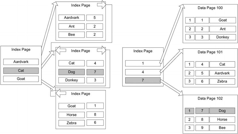
Figure 10-11. Nonclustered index on a clustered table
The overhead of the operation I’ve just described is minimal as long as you keep your clustering key optimal and the index maintained. While having to scan two indexes is more work than just having a pointer to the physical location you have to think of the overall picture. Overall, it’s better than having direct pointers to the table, because only minimal reorganization is required for any modification of the values in the table. Consider if you had to maintain a book index manually. If you used the book page as the way to get to an index value, if had to add a page to the book in the middle you would have to update all of the page numbers. But if all of the topics were ordered alphabetically, and you just pointed to the topic name adding a topic would be easy.
The same is true for SQL Server and the structures can be changed thousands of times a second or more. Since there is very little hardware-based information lingering in the structure, data movement is easy for the query processor, and maintaining indexes is an easy operation. Early versions of SQL Server used physical location pointers, and this led to all manners of corruption in our indexes and tables. And let’s face it, the people with better understanding of such things also tell us that when the size of the clustering key is adequately small, this method is remarkably faster overall than having pointers directly to the table.
The primary benefit of the key structure becomes more obvious when we talk about modification operations. Because the clustering key is the same regardless of physical location, only the lowest level of the clustered index need know where the physical data is. Add to this that the data is organized sequentially, and the overhead of modifying indexes is significantly lowered making all of the data modification operations far faster. Of course, this benefit is only true if the clustering key rarely, or never, changes. Therefore, the general suggestion is to make the clustering key a small nonchanging value, such as an identity column (but the advice section is still a few pages away).
Nonclustered Indexes on a Heap
If a table does not have a clustered index, the table is physically referred to as a heap. One definition of a heap is “a group of things placed or thrown one on top of the other.” This is a great way to explain what happens in a table when you have no clustered index: SQL Server simply puts every new row on the end of the last page for the table. Once that page is filled up, it puts a data on the next page or a new page as needed.
When building a nonclustered index on a heap, the row locator is a pointer to the physical page and row that contains the row. As an example, take the example structure from the previous section with a nonclustered index on the name column of an animal table, represented in Figure 10-12.
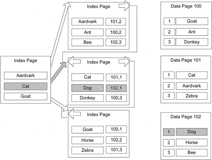
Figure 10-12. Nonclustered index on a heap
If you want to find the row where name ='Dog', you first find the path through the index from the top-level page to the leaf page. Once you get to the leaf page, you get a pointer to the page that has a row with the value, in this case Page 102, Row 1. This pointer consists of the page location and the record number on the page to find the row values (the pages are numbered from 0, and the offset is numbered from 1). The most important fact about this pointer is that it points directly to the row on the page that has the values you’re looking for. The pointer for a table with a clustered index (a clustered table) is different, and this distinction is important to understand because it affects how well the different types of indexes perform.
To avoid the types of physical corruption issues that, as I mentioned in the previous section, can occur when you are constantly managing pointers and physical locations, heaps use a very simple method of keeping the row pointers from getting corrupted. Instead of reordering pages, or changing pointers if the page must be split, it moves rows to a different page and a forwarding pointer is left to point to the new page where the data is now. So if the row where name ='Dog' had moved (for example, due to a large varchar(3000) column being updated from a data length of 10 to 3,000), you might end up with following situation to extend the number of steps required to pick up the data. In Figure 10-13, a forwarding pointer is illustrated.
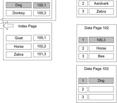
Figure 10-13. Fowarding pointer
All existing indexes that have the old pointer simply go to the old page and follow the forwarding pointer on that page to the new location of the data. If you are using heaps, which should be rare, it is important to be careful with your structures to make sure that data should rarely be moved around within a heap. For example, you have to be careful if you’re often updating data to a larger value in a variable length column that’s used as an index key, it’s possible that a row may be moved to a different page. This adds another step to finding the data, and if the data is moved to a page on a different extent, another read to the database. This forwarding pointer is immediately followed when scanning the table, causing possible horrible performance over time if it’s not managed.
Space is not reused in the heap without rebuilding the table (by selecting into another table, adding a clustered index temporarily, or in 2008, using the ALTER TABLE command with the REBUILD option). In the last section of this chapter on Indexing Dynamic Management View queries, I will provide a query that will give you information on the structure of your index, including the count of forwarding pointers in your table.
The basic syntax for creating an index is as follows:
CREATE [UNIQUE] INDEX [CLUSTERED | NONCLUSTERED] <indexName>
ON <tableName> (<columnList>);
As you can see, you can specify either a clustered or nonclustered index, with nonclustered being the default type. (Recall that the default index created for a primary key constrant is a clustered index.) Each type of index can be unique or nonunique. If you specify that your index must be unique, every row in the indexed column must have a different value—no duplicate entries are accepted, just like one of the uniqueness constraints.
The <columnList> is a comma-delimited list of columns in the table. Each column can be specified either in ascending (ASC) or descending (DESC) order for each column, with ascending being the default. SQL Server can traverse the index in either direction for searches, so the direction is generally only important when you have multiple columns in the index.
For example, the following statement creates an index called XtableA_column1AndColumn2 on column1 and column2 of tableA, with ascending order for column1 and descending order for column2:
CREATE INDEX XtableA_column1AndColumn2 ON tableA (column1, column2 DESC);
Let’s take a look at a more detailed example. First, we need to create a base table. Use whatever database you desire. I used tempdb on my test machine and included the USE statement in the code download.
CREATE SCHEMA produce;
GO
CREATE TABLE produce.vegetable
(
--PK constraint defaults to clustered
vegetableId int NOT NULL CONSTRAINT PKproduce_vegetable PRIMARY KEY,
name varchar(15) NOT NULL
CONSTRAINT AKproduce_vegetable_name UNIQUE,
color varchar(10) NOT NULL,
consistency varchar(10) NOT NULL,
filler char(4000) default (replicate('a', 4000)) NOT NULL
);
![]() Note I included a huge column in the produce table to exacerbate the issues with indexing the table in lieu of having tons of rows to work with. This causes the data to be spread among several data pages, and as such, forces some queries to perform more like a table with a lot more data. I will not return this filler column or acknowledge it much in the chapter, but this is its purpose. Obviously, creating a filler column is not a performance tuning best practice, but it is a common trick to force a table’s data pages to take up more space in a demonstration.
Note I included a huge column in the produce table to exacerbate the issues with indexing the table in lieu of having tons of rows to work with. This causes the data to be spread among several data pages, and as such, forces some queries to perform more like a table with a lot more data. I will not return this filler column or acknowledge it much in the chapter, but this is its purpose. Obviously, creating a filler column is not a performance tuning best practice, but it is a common trick to force a table’s data pages to take up more space in a demonstration.
Now, we create two single-column nonclustered indexes on the color and consistency columns, respectively:
CREATE INDEX Xproduce_vegetable_color ON produce.vegetable(color);
CREATE INDEX Xproduce_vegetable_consistency ON produce.vegetable(consistency);
Then, we create a unique composite index on the vegetableID and color columns. We make this index unique, not to guarantee uniqueness of the values in the columns but because the values in vegetableId must be unique because it’s part of the PRIMARY KEY constraint. Making this unique signals to the optimizer that the values in the index are unique (note that this index is probably not very useful in reality but is created to demonstrate a unique index that isn’t a constraint).
CREATE UNIQUE INDEX Xproduce_vegetable_vegetableId_color
ON produce.vegetable(vegetableId, color);
Finally, we add some test data:
INSERT INTO produce.vegetable(vegetableId, name, color, consistency)
VALUES (1,'carrot','orange','crunchy'), (2,'broccoli','green','leafy'),
(3,'mushroom','brown',’squishy'), (4,'pea','green',’squishy'),
(5,'asparagus','green','crunchy'), (6,’sprouts','green','leafy'),
(7,'lettuce','green','leafy'),( 8,'brussels sprout','green','leafy'),
(9,’spinach','green','leafy'), (10,'pumpkin','orange',’solid'),
(11,'cucumber','green',’solid'), (12,'bell pepper','green',’solid'),
(13,’squash','yellow',’squishy'), (14,'canteloupe','orange',’squishy'),
(15,'onion','white',’solid'), (16,'garlic','white',’solid'),
To see the indexes on the table, we check the following query:
SELECT name, type_desc, is_unique
FROM sys.indexes
WHERE OBJECT_ID('produce.vegetable') = object_id;
This returns the following results:
| name | type_desc | is_unique |
| ========= | ------------- | ------------- |
| PKproduce_vegetable | CLUSTERED | 1 |
| AKproduce_vegetable_name | NONCLUSTERED | 1 |
| Xproduce_vegetable_color | NONCLUSTERED | 0 |
| Xproduce_vegetable_consistency | NONCLUSTERED | 0 |
| Xproduce_vegetable_vegetableId_color | NONCLUSTERED | 1 |
One thing to remind you here is that PRIMARY KEY and UNIQUE constraints were implemented behind the scenes using indexes. The PK constraint is, by default, implemented using a clustered index and the UNIQUE constraint via a nonclustered index. As the primary key is generally chosen to be an optimally small value, it tends to make a nice clustering key.
![]() Note Foreign key constraints aren’t automatically implemented using an index, though indexes on migrated foreign key columns are often useful for performance reasons. I’ll return to this topic later when I discuss the relationship between foreign keys and indexes.
Note Foreign key constraints aren’t automatically implemented using an index, though indexes on migrated foreign key columns are often useful for performance reasons. I’ll return to this topic later when I discuss the relationship between foreign keys and indexes.
The remaining entries in the output show the three nonclustered indexes that we explicitly created and that the last index was implemented as unique since it included the unique key values as one of the columns. Before moving on, briefly note that to drop an index, use the DROP INDEX statement, like this one to drop the Xproduce_vegetable_consistency index we just created:
DROP INDEX Xproduce_vegetable_consistency ON produce.vegetable;
One last thing I want to mention on the basic index creation is a feature that was new to 2008. That feature is the ability to create filtered indexes. By including a WHERE clause in the CREATE INDEX statement, you can restrict the index such that the only values that will be included in the leaf nodes of the index are from rows that meet the where clause. We built a filtered index back in Chapter 8 when I introduced selective uniqueness, and I will mention them again in this chapter to show how to optimize for certain WHERE clauses.
The options I have shown so far are clearly not all of the options for indexes in SQL Server, nor are these the only types of indexes available. For example, there are options to place indexes on different filegroups from tables. Also at your disposal are filestream data (mentioned in Chapter 8), data compression, setting the maximum degree of parallelism to use with an index, locking (page or row locks), rebuilding, and several other features. There are also XML, spatial index types, and as previously mentioned, columnstore indexes. This book focuses specifically on relational databases, so relational indexes are really all that I am covering in any depth.
Basic Index Usage Patterns
In this section, I’ll look at some of the basic usage patterns of the different index types, as well as how to see the use of the index within a query plan:
- Clustered indexes: I’ll discuss the choices you need to make when choosing the columns in which to put the clustered index.
- Nonclustered indexes: After the clustered index is applied, you need to decide where to apply nonclustered indexes.
- Unique indexes: I’ll look at why it’s important to use unique indexes as frequently as possible.
All plans that I present will be obtained using the SET SHOWPLAN_TEXT ON statement. When you’re doing this locally, it can be easier to use the graphical showplan from Management Studio. However, when you need to post the plan or include it in a document, use one of the SET SHOWPLAN_TEXT commands. You can read about this more in SQL Server Books Online. Note that using SET SHOWPLAN_TEXT (or the other versions of SET SHOWPLAN that are available, such as SET SHOWPLAN_XML), do not actually execute the statement/batch; rather, they show the estimated plan. If you need to execute the statement (like to get some dynamic SQL statements to execute to see the plan), you can use SET STATISTICS PROFILE ON to get the plan and some other pertinent information about what has been executed. Each of these session settings will need to be turned OFF explicitly once you have finished, or they will continue executing returning plans where you don’t want so.
For example, say you execute the following query:
SET SHOWPLAN_TEXT ON;
GO
SELECT *
FROM produce.vegetable;
GO
SET SHOWPLAN_TEXT OFF;
GO
Running these statements echoes the query as a single column result set of StmtText and then returns another with the same column name that displays the plan:
|--Clustered Index Scan(OBJECT:([tempdb].[produce].[vegetable].[PKproduce_vegetable]))
Although this is the best way to communicate the plan in text (for example, to post to the MSDN/TechNet or any other forums to get help on why your query is so slow), it is not the richest or easiest experience. In SSMS, click the Query menu and choose Display Estimated Execution Plan (Ctrl+L); you’ll see the plan in a more interesting way, as shown in Figure 10-14. Or by choosing Include Actual Execution Plan, you can see exactly what SQL Server did (which is analogous to SET STATISTICS PROFILE ON).
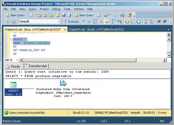
Figure 10-14. Plan display in Management Studio
Before breaking down the different index types, we need to start out by introducing a few terms need to be introduced:
- Scan : This refers to an unordered search, where SQL Server scans the leaf pages of the index looking for a value. Generally speaking, all leaf pages would be considered in the process.
- Seek : This refers to an ordered search, in that the index pages are used to go to a certain point in the index and then a scan is done on a range of values. For a unique index, this would always return a single value.
- Lookup : The clustered index is used to look up a value for the nonclustered index.
Each of these types of operations is very important in understanding how an index is used in a query. Seeks are generally best; scans are less desirable. Lookups aren’t necessarily bad, but too many lookups can be indicative of needing some tuning (often using covering indexes, a topic we will cover in a bit.)
Using Clustered Indexes
The column you use for the clustered index will (because the key is used as the row locator), become a part of every index for your table, so it has heavy implications for all indexes. Because of this, for a typical OLTP system, a very common practice is to choose a surrogate key value, often the primary key of the table, since the surrogate can be kept very small.
Using the surrogate key as the clustering key is usually a great decision, not only because is it a small key (most often, the datatype is an integer that requires only 4 bytes or possibly less using compression), but because it’s always a unique value. As mentioned earlier, a nonunique clustering key has a 4-byte uniquifier tacked onto its value when keys are not unique. It also helps the optimizer that an index has only unique values, because it knows immediately that for an equality operator, either 1 or 0 values will match. Because the surrogate key is often used in joins, it’s helpful to have smaller keys for the primary key.
![]() Caution Using a GUID for a surrogate key is becoming the vogue these days, but be careful. GUIDs are 16 bytes wide, which is a fairly large amount of space, but that is really the least of the problem. They are random values, in that they generally aren’t monotonically increasing, and a new GUID could sort anywhere in a list of other GUIDs.
Caution Using a GUID for a surrogate key is becoming the vogue these days, but be careful. GUIDs are 16 bytes wide, which is a fairly large amount of space, but that is really the least of the problem. They are random values, in that they generally aren’t monotonically increasing, and a new GUID could sort anywhere in a list of other GUIDs.
Clustering on a random value is generally troublesome for inserts, because if you don’t leave spaces on each page for new rows, you are likely to have page splitting. If you have a very active system, the constant page splitting can destroy your system, and the opposite effect, to leave lots of empty space, can be just as painful, as you make reads far less effective. The only way to make GUIDs a reasonably acceptable type is to use the NEWSEQUENTIALID() function (or one of your own) to build sequential GUIDS, but it only works with unique identifier columns in a default constraint. Seldom will the person architecting a solution that is based on GUID surrogates want to be tied down to using a default constraint to generate surrogate values. The ability to generate GUIDs from anywhere and ensure their uniqueness is part of the lure of the siren call of the 16-byte value. For SQL Server 2012, the use of the sequence object to generate guaranteed unique values could be used in lieu of GUIDs.
The clustered index won’t always be used for the surrogate key or even the primary key. Other possible uses can fall under the following types:
- Range queries : Having all the data in order usually makes sense when there’s data that you often need to get a range, such as from A to F. An example where this can make sense is for the child rows in a parent child relationship.
- Data that’s always accessed sequentially: Obviously, if the data needs to be accessed in a given order, having the data already sorted in that order will significantly improve performance.
- Queries that return large result sets: This point will make more sense once I cover nonclustered indexes, but for now, note that having the data on the leaf index page saves overhead.
The choice of how to pick the clustered index depends on a couple factors, such as how many other indexes will be derived from this index, how big the key for the index will be, and how often the value will change. When a clustered index value changes, every index on the table must also be touched and changed, and if the value can grow larger, well, then we might be talking page splits. This goes back to understanding the users of your data and testing the heck out of the system to verify that your index choices don’t hurt overall performance more than they help. Speeding up one query by using one clustering key could hurt all queries that use the nonclustered indexes, especially if you chose a large key for the clustered index.
Frankly, in an OLTP setting, in all but the most unusual cases, I stick with a surrogate key for my clustering key, usually one of the integer types or sometimes even the uniqueidentifier (GUID) type (ideally the sequential type). I use the surrogate key because so many of the queries you do for modification (the general goal of the OLTP system) will access the data via the primary key. You then just have to optimize retrievals, which should also be of generally small numbers of rows, and doing so is usually pretty easy.
Another thing that is good about using the clustered index on a monotonically increasing value is that page splits over the entire index are greatly decreased. The table grows only on one end of the index, and while it does need to be rebuilt occasionally using ALTER INDEX REORGANIZE or ALTER INDEX REBUILD, you don’t end up with page splits all over the table. You can decide which to do by using the criteria stated by SQL Server Books Online. By looking in the dynamic management view sys.dm_db_index_physical_stats, you can use REBUILD on indexes with greater than 30% fragmentation and use REORGANIZE otherwise. Now, let’s look at an example of a clustered index in use. If you have a clustered index on a table, instead of Table Scan, you’ll see a Clustered Index Scan in the plan:
SELECT *
FROM produce.vegetable;
The plan for this query is as follows:
|--Clustered Index Scan(OBJECT:([tempdb].[produce].[vegetable].[PKproduce_vegetable]))
If you query on a value of the clustered index key, the scan will likely change to a seek. Although a scan touches all the data pages, a clustered index seek uses the index structure to find a starting place for the scan and knows just how far to scan. For a unique index with an equality operator, a seek would be used to touch one page in each level of the index to find (or not find) a single value on a single data page, for example:
SELECT *
FROM produce.vegetable
WHERE vegetableId = 4;
The plan for this query now does a seek:
|--Clustered Index Seek(OBJECT:([tempdb].[produce].[vegetable].[PKproduce_vegetable]),
SEEK:([tempdb].[produce].[vegetable].[vegetableId]=
CONVERT_IMPLICIT(int,[@1],0)) ORDERED FORWARD)
Note the CONVERT_IMPLICIT of the @1 value. This shows the query is being parameterized for the plan, and the variable is cast to an integer type. In this case, you’re seeking in the clustered index based on the SEEK predicate of vegetableId = 4. SQL Server will create a reusable plan by default for simple queries. Any queries that are executed with the same exact format, and a simple integer value would use the same plan. You can let SQL Server paramaterize more complex queries as well. (For more information, look up “Simple Paramaterization and Forced Parameterization” in Books Online.) Increasing the complexity, now, we search for two rows:
SELECT *
FROM produce.vegetable
WHERE vegetableId in (1,4);
And in this case, pretty much the same plan is used, except the seek criteria now has an OR in it:
|--Clustered Index Seek(OBJECT:([tempdb].[produce].[vegetable].[PKproduce_vegetable]),
SEEK:([tempdb].[produce].[vegetable].[vegetableId]=(1)
OR [tempdb].[produce].[vegetable].[vegetableId]=(4)) ORDERED FORWARD)
Note that it did not create a parameterized plan this time, but a fixed one with literals for 1 and 4. Note that this plan will be executed as two separate seek operations. If you turn on SET STATISTICS IO before running the query:
SET STATISTICS IO ON;
GO
SELECT *
FROM produce.vegetable
WHERE vegetableId in (1,4);
Go
SET STATISTICS IO OFF;
You will see that it did two “scans”, which using STATISTICS IO generally means any operation that probes the table, so a seek or scan would show up the same (note the lob values are for large objects such as (max) types):
Table 'vegetable'. Scan count 2, logical reads 4, physical reads 0, read-ahead reads 0, lob logical reads 0, lob physical reads 0, lob read-ahead reads 0.
But whether any given query uses a seek or scan, or even two seeks, can be a pretty complex question. Why it is so complex will become clearer over the rest of the chapter, and it will become instantly clearer how useful a clustered index seek is in the next section, “Using Nonclustered Indexes.”
A final consideration you need to think about is how the index will be used. There are two types of index usages, equality and inequality. In a query such as the previous ones, we have done as the following:
SELECT *
FROM produce.vegetable
WHERE vegetableId = 4;
Or even the queries with the IN Boolean expression, these have been equality operators, where the values that were being searched for were known at compile time. For inequality searches, you will look for a value greater than some other value, or between values. So for this query, it has the following plan:
|--Clustered Index Seek(OBJECT:([tempdb].[produce].[vegetable].[PKproduce_vegetable]),
SEEK:([tempdb].[produce].[vegetable].[vegetableId]=
CONVERT_IMPLICIT(int,[@1],0)) ORDERED FORWARD)
Changing this to an inequality search, such as
SELECT *
FROM produce.vegetable
WHERE vegetableId > 4;
Now, you will get the following plan:
|--Clustered Index Seek(OBJECT:([tempdb].[produce].[vegetable].[PKproduce_vegetable]),
SEEK:([tempdb].[produce].[vegetable].[vegetableId] > (4)) ORDERED FORWARD)
Note that, this time, even though we did a fairly simple query, it did not automatically parameterize. This is because the plan can change drastically based on the value passed.
Using Nonclustered Indexes
After you have made the ever-important choice of what to use for the clustered index, all other indexes will be nonclustered. In this section, I will cover nonclustered indexes in the following areas:
- General considerations
- Composite index considerations
- Nonclustered indexes with clustered tables
- Nonclustered indexes on heaps
General Considerations
We generally know that indexes are needed because queries are slow. Lack of indexes is clearly not the only reason that queries are slow. Here are some of the obvious reasons for slow queries:
- Extra heavy user load
- Hardware load
- Network load
After looking for the existence of the preceding reasons, we can pull out Management Studio and start to look at the plans of the slow queries. Most often, slow queries are apparent because either |--Clustered Index Scan or |--Table Scan shows up in the query plan, and those operations take a large percentage of time to execute. Simple, right? Essentially, it is a true enough statement that index and table scans are time consuming, but unfortunately, that really doesn’t give a full picture of the process. It’s hard to make specific indexing changes before knowing about usage, because the usage pattern will greatly affect these decisions, for example:
- Is a query executed once a day, once an hour, or once a minute?
- Is a background process inserting into a table rapidly? Or perhaps inserts are taking place during off hours?
Using Profiler and the Dynamic Management Views, you can watch the usage patterns of the queries that access your database, looking for slowly executing queries, poor plans, and so on. After you do this and you start to understand the usage patterns for your database, you now need to use that information to consider where to apply indexes—the final goal being that you use the information you can gather about usage and tailor an index plan to solve the overall picture.
You can’t just throw around indexes to fix individual queries. Nothing comes without a price, and indexes definitely have a cost. You need to consider how indexes help and hurt the different types of operations in different ways:
- SELECT : Indexes can only have a beneficial effect on SELECT queries.
- INSERT : An index can only hurt the process of inserting new data into the table. As data is created in the table, there’s a chance that the index will have to be modified and reorganized to accommodate the new values.
-
UPDATE
: An update requires two or three steps: find the row(s) and change the row(s), or find the row(s), delete them, and reinsert them. During the phase of finding the row, the index is beneficial, such as for a SELECT. Whether or not it hurts during the second phase depends on several factors, for example:
- Did the index key value change such that it needs to be moved around to different leaf nodes?
- Will the new value fit on an existing page, or will it require a page split? (More on that later in this section.)
- DELETE : The delete requires two steps: to find the row and to remove it. Indexes are beneficial to find the row, but on deletion, you might have to do some reshuffling to accommodate the deleted values from the indexes.
You should also realize that for INSERT, UPDATE, or DELETE operations, if triggers on the table exist (or constraints exist that execute functions that reference tables), indexes will affect those operations in the same ways as in the list. For this reason, I’m going to shy away from any generic advice about what types of columns to index. In practice, there are just too many variables to consider.
![]() Tip Too many people index without considering the costs. Just be wary that every index you add has to be maintained. Sometimes, a query taking 1 second to execute is OK when getting it down to .1 seconds might slow down other operations considerably. The real question lies in how often each operation occurs and how much cost you are willing to suffer. The hardest part is keeping your tuning hat off until you can really get a decent profile of what operations are taking place.
Tip Too many people index without considering the costs. Just be wary that every index you add has to be maintained. Sometimes, a query taking 1 second to execute is OK when getting it down to .1 seconds might slow down other operations considerably. The real question lies in how often each operation occurs and how much cost you are willing to suffer. The hardest part is keeping your tuning hat off until you can really get a decent profile of what operations are taking place.
For a good idea of how your current indexes and/or tables are currently being used, you can query the dynamic management view sys.dm_db_index_usage_stats:
SELECT OBJECT_NAME(i.object_id) as object_name
, CASE WHEN i.is_unique = 1 THEN 'UNIQUE ' ELSE '' END +
i.TYPE_DESC as index_type
, i.name as index_name
, user_seeks, user_scans, user_lookups,user_updates
FROM sys.indexes i
LEFT OUTER JOIN sys.dm_db_index_usage_stats AS s
ON i.object_id = s.object_id
AND i.index_id = s.index_id
AND database_id = db_id()
WHERE OBJECTPROPERTY(i.object_id , 'IsUserTable') = 1
ORDER BY 1,3;
This query will return the name of each object, an index type, an index name, plus the number of
- User seeks : The number of times the index was used in a seek operation
- User scans : The number of times the index was scanned in answering a query
- User lookups : For clustered indexes, the number of times the index was used to resolve the row locator of a nonclustered index search
- User updates : The number of times the index was changed by a user query
This information is very important when trying to get a feel for which indexes might need to be tuned and especially which ones are not doing their jobs, because they are mostly getting updated. You could probably boil performance tuning to a math equation if you had an advanced degree in math and a lot of time, but truthfully, it would take longer than just testing in most cases, especially if you have a good performance-testing plan for your system. Even once you know the customer’s answer to these questions, you should test your database code on your performance-testing platform. Performance testing is a tricky art, but it doesn’t usually take tremendous amounts of time to identify your hot spots and optimize them, and to do the inevitable tuning of queries in production.
Determining Index Usefulness
It might seem at this point that all you need to do is look at the plans of queries, look for the search arguments, and put an index on the columns, so things will improve. There’s a bit of truth to this, but indexes have to be useful to be used by a query. What if the index of a 418-page book had two entries:
- General Topics 1
- Determining Index Usefulness 417
This means that one page was classified such that the topic started on this page, and all other pages covered general topics. This would be useless to you, unless you needed to know about indexes. One thing is for sure: you could determine that the index was useless pretty quickly. Another thing we all do with the index of a book to see if it’s useful is to take a value and look it up in the index. If what you’re looking for is in there (or something close), you go to the page and check it out.
SQL Server determines whether or not to use your index in much the same way. It has two specific measurements that it uses to decide if an index is useful: the density of values (sometimes known as the selectivity) and a histogram of a sample of values in the table to check against.
You can see these in detail for indexes by using DBCC SHOW_STATISTICS . Our table is very small, so it doesn’t need stats to decide which to use. Instead, we’ll look at an index in the AdventureWorks2012 database:
DBCC SHOW_STATISTICS('AdventureWorks2012.Production.WorkOrder',
'IX_WorkOrder_ProductID') WITH DENSITY_VECTOR;
DBCC SHOW_STATISTICS('AdventureWorks2012.Production.WorkOrder',
'IX_WorkOrder_ProductID') WITH HISTOGRAM;
This returns the following sets (truncated for space). The first tells us the size and density of the keys. The second shows the histogram of where the table was sampled to find representative values.
| All density | Average Length | Columns |
| ----------- | ------------- | ------------- |
| 0.004201681 | 4 | ProductID |
| 1.377581E-05 | 8 | ProductID, WorkOrderID |
| RANGE_HI_KEY | RANGE_ROWS | EQ_ROWS | DISTINCT_RANGE_ROWS | AVG_RANGE_ROWS |
| ------------- | ------------- | ------------- | ------------- | ------------- |
| 3 | 0 | 1093 | 0 | 1 |
| 316 | 0 | 1093 | 0 | 1 |
| 324 | 0 | 1093 | 0 | 1 |
| 327 | 0 | 1093 | 0 | 1 |
| ... | ... | ... | ... | ... |
| 994 | 0 | 878 | 0 | 1 |
| 995 | 0 | 710 | 0 | 1 |
| 996 | 0 | 1084 | 0 | 1 |
| 997 | 0 | 236 | 0 | 1 |
| 998 | 0 | 236 | 0 | 1 |
| 999 | 0 | 233 | 0 | 1 |
I won’t cover the DBCC SHOW_STATISTICS command in great detail, but there are a couple important things to understand. First, consider the density of each column set. The ProductId column is the only column that is actually declared in the index, but note that it includes the density of the index column and the clustered index key as well (it’s known as the clustering key , which I’ll cover more later in this chapter).
All the density is calculated approximately by 1 / number of distinct rows, as shown here for the same columns as I just checked the density on:
--Used isnull as it is easier if the column can be null
--value you translate to should be impossible for the column
--ProductId is an identity with seed of 1 and increment of 1
--so this should be safe (unless a dba does something weird)
SELECT 1.0/COUNT(DISTINCT ISNULL(ProductID,-1)) AS density,
COUNT(DISTINCT ISNULL(ProductID,-1)) AS distinctRowCount,
1.0/count(*) as uniqueDensity,
COUNT(*) as allRowCount
FROM AdventureWorks2012.Production.WorkOrder;
This returns the following:
density distinctRowCount uniqueDensit yallRowCount
------------ ------------- ----------------- -------------------
0.004201680672 2380 .000013775812 72591
You can see that the densities match. (The queries density is in a numeric type, while the DBCC is using a float, which is why they are formatted differently, but they are the same value!) The smaller the number, the better the index, and the more likely it will be easily chosen for use. There’s no magic number, per se, but this value fits into the calculations of which way is best to execute the query. The actual numbers returned from this query might vary slightly from the DBCC value, as a sampled number might be used for the distinct count.
The second thing to understand in the DBCC SHOW_STATISTICS output is the histogram. Even if the density of the index isn’t low, SQL Server can check a given value (or set of values) in the histogram to see how many rows will likely be returned. SQL Server keeps statistics about columns in a table as well as in indexes, so it can make informed decisions as to how to employ indexes or table columns. For example, consider the following rows from the histogram (I have faked some of these results for demonstration purposes):
| RANGE_HI_KEY | RANGE_ROWS | EQ_ROWS | DISTINCT_RANGE_ROWS | AVG_RANGE_ROWS |
| ------------- | ------------- | ------------- | ------------- | ------------- |
| ... | ... | ... | ||
| 989 | 111 | 58 | 2 | 55.5 |
| 992 | 117 | 67 | 2 | 58.5 |
In the second row, the row values tell us the following:
- RANGE_HI_KEY : The sampled ProductId values were 989 and 992.
- RANGE_ROWS : There are 117 rows where the value was between 989 and 992 (noninclusive of the endpoints). These values would not be known. However, if a user used 990 as a search argument, the optimizer can now know that a maximum of 117 rows would be returned. This is one of the ways that the query plan gets the estimated number of rows for each step in a query and is one of the ways to determine if an index will be useful for an individual query.
- EQ_ROWS : There were exactly 67 rows where ProductId = 992.
- DISTINCT_RANGE_ROWS : For the row with 989, it is estimated that there are two distinct values between 989 and 992.
- AVG_RANGE_ROWS : This is the average number of duplicate values in the range, excluding the upper and lower bounds. This value is what the optimizer can expect to be the average number of rows. Note that this is calculated by RANGE_ROWS / DISTINCT_RANGE_ROWS.
One thing that having this histogram can do is allow a seemingly useless index to become valuable in some cases. For example, say you want to index a column with only two values. If the values are evenly distributed, the index would be useless. However, if there are only a few of a certain value, it could be useful (going back to the tempdb):
(
testIndex int NOT NULL IDENTITY(1,1) CONSTRAINT PKtestIndex PRIMARY KEY,
bitValue bit NOT NULL,
filler char(2000) NOT NULL DEFAULT (replicate('A',2000)) NOT NULL
);
CREATE INDEX XtestIndex_bitValue ON testIndex(bitValue);
GO
SET NOCOUNT ON;
INSERT INTO testIndex(bitValue)
VALUES (0);
GO 50000 --runs current batch 50000 times in Management Studio.
INSERT INTO testIndex(bitValue)
VALUES (1);
GO 100 --puts 100 rows into table with value 1
You can guess that few rows will be returned if the only value desired is 1. Check the plan for bitValue = 0 (again using SET SHOWPLAN ON, or using the GUI):
SELECT *
FROM testIndex
WHERE bitValue = 0;
This shows a clustered index scan:
|--Clustered Index Scan(OBJECT:([tempdb].[dbo].[testIndex].[PKtestIndex]),
WHERE:([tempdb].[dbo].[testIndex].[bitValue]=(0)))
However, change the 0 to a 1, and the optimizer chooses an index seek. This means that it performed a seek into the index to the first row that had a 1 as a value and worked its way through the values:
|--Nested Loops(Inner Join, OUTER REFERENCES:
([tempdb].[dbo].[testIndex].[testIndex], [Expr1003]) WITH UNORDERED PREFETCH)
|--Index Seek(OBJECT:([tempdb].[dbo].[testIndex].[XtestIndex_bitValue]),
SEEK:([tempdb].[dbo].[testIndex].[bitValue]=(1)) ORDERED FORWARD)
|--Clustered Index Seek(OBJECT:([tempdb].[dbo].[testIndex].[PKtestIndex]),
SEEK:([tempdb].[dbo].[testIndex].[testIndex]=
[tempdb].[dbo].[testIndex].[testIndex]) LOOKUP ORDERED FORWARD)
This output may look a bit odd, but this plan shows that the query processor will do the index seek to find the rows that match and then a nested loop join to the clustered index to get the rest of the data for the row (because we chose to do SELECT *), getting the entire data row (more on how to avoid the clustered seek in the next section).
You can see why in the histogram:
UPDATE STATISTICS dbo.testIndex;
DBCC SHOW_STATISTICS('dbo.testIndex', 'XtestIndex_bitValue') WITH HISTOGRAM;
This returns the following results (your actual values will likely vary, and in fact, in some tests, only the 0 rows showed up in the output):
| RANGE_HI_KEY | RANGE_ROWS | EQ_ROWS | DISTINCT_RANGE_ROWS | AVG_RANGE_ROWS |
| ------------- | ------------- | ------------- | ------------- | ------------- |
| 0 | 0 | 49976.95 | 0 | 1 |
| 1 | 0 | 123.0454 | 0 | 1 |
The statistics gathered estimated that about 123 rows match for bitValue = 1. That’s because statistics gathering isn’t an exact science—it uses a sampling mechanism rather than checking every value (your values might vary as well). Check out the TABLESAMPLE clause, and you can use the same mechanisms to gather random samples of your data.
The optimizer knew that it would be advantageous to use the index when looking for bitValue = 1, because approximately 123 rows are returned when the index key with a value of 1 is desired, but 49,977 are returned for 0. (Your try will likely return a different value. For the rows where the bitValue was 1, I got 80 in the previous edition and 137 in a different set of tests. They are all approximately the 100 that you should expect, since we specifically created 100 rows when we loaded the table.)
This demonstration of the histogram is good, but in practice, starting in SQL Server 2008, actually building a filtered index to optimize this query may be a better practice. You might build an index such as this:
CREATE INDEX XtestIndex_bitValueOneOnly
ON testIndex(bitValue) WHERE bitValue = 1;
The histogram for this index is definitely by far a clearer good match:
| RANGE_HI_KEY | RANGE_ROWS | EQ_ROWS | DISTINCT_RANGE_ROWS | AVG_RANGE_ROWS |
| ------------- | ------------- | ------------- | ------------- | ------------- |
| 1 | 0 | 100 | 0 | 1 |
Whether or not the query actually uses this index will likely depend on how badly the other index would perform, which can also be dependent on hardware conditions. A histogram is, however, another tool that you can use when optimizing your SQL to see what the optimizer is using to make its choices.
![]() Tip Whether or not the histogram includes any data where the bitValue = 1 is largely a matter of chance. I have run this example several times, and one time, no rows were shown unless I used the FULLSCAN option on the UPDATE STATISTICS command (which isn’t feasible on very large tables unless you have quite a bit of time).
Tip Whether or not the histogram includes any data where the bitValue = 1 is largely a matter of chance. I have run this example several times, and one time, no rows were shown unless I used the FULLSCAN option on the UPDATE STATISTICS command (which isn’t feasible on very large tables unless you have quite a bit of time).
As we discussed in the clustered index section, queries can be for equality or inequality. For equality searches, the query optimizer will use the single point and estimate the number of rows. For inequality, it will use the starting point and ending point of the inequality and determine the number of rows that will be returned from the query.
Indexing and Multiple Columns
So far, the indexes I’ve talked about were mostly on single columns, but it isn’t all that often that you only need performance enhancing indexes on single columns. When multiple columns are included in the WHERE clause of a query on the same table, there are several possible ways you can enhance your queries:
- Having one composite index on all columns
- Creating covering indexes by including all columns that a query touches
- Having multiple indexes on separate columns
- Adjusting key sort order to optimize sort operations
When you include more than one column in an index, it’s referred to as a composite index. As the number of columns grows, the effectiveness of the index is reduced for the general case. The problem is that the index is sorted by the first column values. So the second column in the index is more or less only useful if you need the first column as well. Even so, you will very often need composite indexes to optimize common queries when predicates on all of the columns involved.
The order of the columns in a query is important with respect to whether a composite can and will be used. There are a couple important considerations:
- Which column is most selective? If one column includes unique or mostly unique values, it is possibly a good candidate for the first column. The key is that the first column is the one by which the index is sorted. Searching on the second column only is less valuable (though queries using only the second column can scan the index leaf pages for values).
- Which column is used most often without the other columns? One composite index can be useful to several different queries, even if only the first column of the index is all that is being used in those queries.
For example, consider this query:
SELECT vegetableId, name, color, consistency
FROM produce.vegetable
WHERE color = 'green'
AND consistency = 'crunchy';
An index on color or consistency alone might not do the job well enough (of course, it will in this case, as vegetable is a very small table). If the plan that is being produced by the optimizer is to do a table scan, you might consider adding a composite index on color and consistency. This isn’t a bad idea to consider, and composite indexes are great tools, but just how useful such an index will be is completely dependent on how many rows will be returned by color = 'green' and consistency = 'crunchy'.
The preceding query with existing indexes (clustered primary key on produceId, alternate key on Name, indexes on color and consistency, plus a composite index on vegetable and color_) is optimized with the following plan:
|--Clustered Index
Scan(OBJECT:([tempdb].[produce].[vegetable].[PKproduce_vegetable]),
WHERE:([tempdb].[produce].[vegetable].[color]='green'
AND [tempdb].[produce].[vegetable].[consistency]='crunchy'))
Adding an index on color and consistency seems like a good way to further optimize the query, but first, you should look at the data for these columns (consider future usage of the index too, but existing data is a good place to start):
SELECT color, consistency, count(*) as [count]
FROM produce.vegetable
GROUP BY color, consistency
ORDER BY color, consistency;
which returns:
| color | consistency | count |
| ------------- | ------------- | ------------- |
| brown | squishy | 1 |
| green | crunchy | 1 |
| green | leafy | 5 |
| green | solid | 2 |
| green | squishy | 1 |
| orange | crunchy | 1 |
| orange | solid | 1 |
| orange | squishy | 1 |
| white | solid | 2 |
| yellow | squishy | 1 |
Of course, you can’t always look at all of the rows like this, so another possibility is to see which of the columns has more distinct values:
SELECT COUNT(DISTINCT color) as color,
COUNT(DISTINCT consistency) as consistency
FROM produce.vegetable;
This query returns the following:
| color | consistency |
| ------------- | ------------- |
| 5 | 4 |
The column consistency has the most unique values (though not tremendously, in real practice, the difference in the number of values will often be much greater). So we add the following index:
CREATE INDEX Xproduce_vegetable_consistencyAndColor
ON produce.vegetable(consistency, color);
The plan changes to the following (well, it would if there were lots more data in the table, so I have forced the plan to generate this particular example; otherwise, because there is such a small amount of data, the clustered index would always be used for all queries):
|--Nested Loops(Inner Join, OUTER REFERENCES:
([tempdb].[produce].[vegetable].[vegetableId]))
|--Index Seek(OBJECT:(
[tempdb].[produce].[vegetable].[Xproduce_vegetable_consistencyAndColor]),
SEEK:([tempdb].[produce].[vegetable].[consistency]='crunchy'
AND [tempdb].[produce].[vegetable].[color]='green') ORDERED FORWARD)
|--Clustered Index Seek(OBJECT:
[tempdb].[produce].[vegetable].[PKproduce_vegetable]),
SEEK:([tempdb].[produce].[vegetable].[vegetableId]=
[tempdb].[produce].[vegetable].[vegetableId]) LOOKUP ORDERED FORWARD)
The execution plan does an index seek on the Xvegetable_consistencyAndColor index, and it uses the clustered index named PKproduce_vegetable to fetch the other parts of the row that were not included in the Xvegetable_consistencyAndColor index. (This is why the clustered index seek is noted as LOOKUP ORDERED FORWARD. In the graphical version of the plan, it will be called a key lookup (clustered) operator).
Keep in mind, too, exactly how the indexes will be used. If your queries mix equality comparisions and inequality comparisons, you will likely want to favor the columns you are using in equality searches first. Of course, your selectivity estimates need to be based on how selective the index will be for your situations. For example, if you are doing small ranges on very selective data in a given column, that could be the best first column in the index. If you have a question about how you think an index can help, test multiple cases and see how the plans and costs change. If you have questions about why a plan is behaving as it is, use the statistics to get more deep ideas about why an index is chosen.
In the next section, I will show how you can eliminate the clustered index scan, but in general, having the scan isn’t the worst thing in the world unless you are matching lots of rows. In this case, for example, the two single-row seeks would result in better performance than a full scan through the table. When the number of rows found using the nonclustered index grows large, however, a plan such as the preceding one can become very costly.
When you are only retrieving data from a table, if an index exists that has all the data values that are needed for a query, the base table needn’t be touched. Back in Figure 10-10, there was a nonclustered index on the type of animal. If the name of the animal was the only data the query needed to touch, the data pages of the table wouldn’t need to be accessed directly. The index covers all the data needed for the query and is commonly referred to as a covering index. The ability to create covering indexes is a nice feature, and the approach even works with clustered indexes, although with clustered indexes, SQL Server scans the lowest index structure page, because scanning the leaf nodes of the clustered index is the same as a table scan.
As a baseline to the example, let’s run the following query:
SELECT name, color
FROM produce.vegetable
WHERE color = 'green';
The resulting plan is a simple clustered index scan:
|--Clustered Index Scan(OBJECT:([tempdb].[produce].[vegetable].[PKproduce_vegetable]),
WHERE:([tempdb].[produce].[vegetable].[color]='green'))
We could do a couple of things to improve the performance of the query. First, we could create a composite index on the color and name columns; it would use the color column to filter the results, and since the name column is in the index, the query processor would never need to go to the base table to get the data to return the results. If you will be filtering on the name column in some cases, that would be the best thing to do.
However, in SQL Server 2005, a new feature was added to the index-creation syntax to improve the ability to implement covering indexes—the INCLUDE (<columns>) clause of the CREATE INDEX statement. The included columns can be almost any datatype, even (max)-type columns. In fact, the only types that aren’t allowed are text, ntext, and image datatypes, but you shouldn’t use these types anyhow, as they’re in the process of being deprecated (you should expect them eventually be completely removed from the product).
Using the INCLUDE keyword gives you the ability to add columns to cover a query without including those columns in the index pages, and thus without causing overhead in the use of the index. Instead, the data in the INCLUDE columns is added only to the leaf pages of the index. The INCLUDE columns won’t help in index seeking, but they do eliminate the need to go to the data pages to get the data being sought.
To demonstrate, let’s modify the index on vegetable color and include the name column:
DROP INDEX Xproduce_vegetable_color ON produce.vegetable;
CREATE INDEX Xproduce_vegetable_color ON produce.vegetable(color) INCLUDE (name);
Now, the query goes back to only touching the index, because it has all the data in the index, and this time, it doesn’t even need to go to the clustered index to pick up the name column:
|--Index Seek(OBJECT:([tempdb].[produce].[vegetable].[Xproduce_vegetable_color]),
SEEK:([tempdb].[produce].[vegetable].[color]=[@1]) ORDERED FORWARD)
This ability to include columns only in the leaf pages of covering indexes is incredibly useful in a lot of situations. Too many indexes with overly large keys are created to cover a query to avoid accessing the base table and end up being only good for one situation, which ends up wasting valuable resources. Now, using INCLUDE, you get the benefits of a covering index without the overhead of bloating the nonleaf pages of the index.
Be careful not to go crazy with covering indexes unless you can see a large benefit from them. The INCLUDE feature costs less to maintain than including the values in the index structure, but it doesn’t make the index structure free to maintain, and it can be very costly to maintain if it references a varchar(max) column, as but one example. One thing you will likely notice when looking at query plans, or the missing index dynamic management views is that indexes using the INCLUDE feature are commonly suggested, because quite often, the key lookup is the most costly part of queries. I must include a caution about going too far and abusing covering indexes, because their use does incur a fairly heavy cost. Be careful to test that the additional overhead of duplicating data in indexes doesn’t harm performance more than it helps it.
Sometimes, we might not have a single index on a table that meets the given situation for the query optimizer to do an optimum job. In this case, SQL Server can sometimes use two or more indexes to meet the need. When processing a query with multiple indexes, SQL Server uses the indexes as if they were tables, joins them together, and returns a set of rows. The more indexes used, the larger the cost, but using multiple indexes can be dramatically faster in some cases.
Multiple indexes aren’t usually something to rely on to optimize known queries. It’s almost always better to support a known query with a single index. However, if you need to support ad hoc queries that cannot be foretold as a system designer, having several indexes that are useful for multiple situations might be the best idea. If you’re building a read-only table, a decent starting strategy might be to index every column that might be used as a filter for a query.
My focus throughout this book has been on OLTP databases, and for that type of database, using multiple indexes in a single query isn’t typical. However, it’s possible that the need for using multiple indexes will arise if you have a table with several columns that you’ll allow users to query against in any combination.
For example, assume you want data from four columns in a table that contains telephone listings. You might create a table for holding phone numbers called phoneListing with these columns: phoneListingId, firstName, lastName, zipCode, areaCode, exchange, and number (assuming United States–style phone numbers).
You have a clustered primary key index on phoneListingId, nonclustered composite indexes on lastName and firstName, one on areaCode and exchange, and another on zipCode. From these indexes, you can effectively perform a large variety of searches, though generally speaking, none of these will be perfect alone, but with one or two columns considered independently, it might be adequate.
For less typical names (such as Leroy Shlabotnik, for example), a person can find this name without knowing the location. For other names, hundreds and thousands of other people have the same first and last names. I always thought I was the only schmuck with the name Louis Davidson, but it turns out that there are quite a few others!
We could build a variety of indexes on these columns, such that SQL Server would only need a single index. However, not only would these indexes have a lot of columns in them but you’d need several indexes. A composite index can be useful for searches on the second and third columns, but if the first column is not included in the filtering criteria, it will require a scan, rather than a seek, of the index. Instead, for large sets, SQL Server can find the set of data that meets one index’s criteria and then join it to the set of rows that matches the other index’s criteria.
This technique can be useful when dealing with large sets of data, especially when users are doing ad hoc querying, and you cannot anticipate what columns they’ll need until runtime. Users have to realize that they need to specify as few columns as possible, because if the multiple indexes can cover a query such as the one in the last section, the indexes will be far more likely to be used.
As an example, we’ll use the data already created, and add an index on the consistency column:
CREATE INDEX Xproduce_vegetable_consistency ON produce.vegetable(consistency);
--existing index repeated as a reminder
--CREATE INDEX Xproduce_vegetable_color ON produce.vegetable(color) INCLUDE (name);
We’ll force the optimizer to use multiple indexes (because the sample table is far too small to require multiple indexes), so we can show how this looks in a plan:
SELECT consistency, color
FROM produce.vegetable with (index=Xproduce_vegetable_color,
index=Xproduce_vegetable_consistency)
WHERE color = 'green'
and consistency = 'leafy';
This produces the following plan:
|--Merge Join(Inner Join, MERGE:([tempdb].[produce].[vegetable].[vegetableId])=
([tempdb].[produce].[vegetable].[vegetableId]),
RESIDUAL:([tempdb].[produce].[vegetable].[vegetableId] =
[tempdb].[produce].[vegetable].[vegetableId]))
|--Index Seek(OBJECT:([tempdb].[produce].[vegetable].[Xproduce_vegetable_color]),
SEEK:([tempdb].[produce].[vegetable].[color]='green') ORDERED FORWARD)
|--Index Seek(OBJECT:
([tempdb].[produce].[vegetable].[Xproduce_vegetable_consistency]),
SEEK:([tempdb].[produce].[vegetable].[consistency]='leafy')
ORDERED FORWARD)
Looking at a snippet of the plan for this query, you can see that there are two index seeks to find rows where color = 'green' and consistency = 'leafy'. These seeks would be fast on even a very large set, as long as the index was reasonably selective. Then, a merge join is done between the sets, because the sets can be ordered by the clustered index. (There’s a clustered index on the table, so the clustering key is included in the index keys.)
While SQL Server can traverse an index in either direction (since it is a doubly linked list), sometimes sorting the keys of an index to match the sort order of some desired output can be valuable. For example, consider the case where you want to look at the hire dates of your employees, in descending order by hire date. To do that, execute the following query (in the AdventureWorks2012 database):
SELECT MaritalStatus, HireDate
FROM Adventureworks2012.HumanResources.Employee
ORDER BY MaritalStatus ASC, HireDate DESC;
The plan for this query follows:
|--Sort(ORDER BY:([AdventureWorks2012].[HumanResources].[Employee].[MaritalStatus] ASC,
[AdventureWorks2012].[HumanResources].[Employee].[HireDate] DESC))
|--Clustered Index Scan(OBJECT:(
[AdventureWorks2012].[HumanResources].[Employee].[PK_Employee_BusinessEntityID]))
Next, create a typical index with the default (ascending) sort order:
CREATE INDEX Xemployee_maritalStatus_hireDate ON
Adventureworks2012.HumanResources.Employee (MaritalStatus,HireDate);
Rechecking the plan, you will see that the plan changes to an index scan (since it can use the index to cover the query), but it still requires a sort operation.
|--Sort(ORDER BY:([AdventureWorks2012].[HumanResources].[Employee].[MaritalStatus] ASC,
AdventureWorks2012].[HumanResources].[Employee].[HireDate] DESC))
|--Index Scan(OBJECT: ([AdventureWorks2012].[HumanResources].[Employee].
[Xemployee_maritalStatus_hireDate]))
That’s better but still not quite what we want. Change the index we just added to be sorted in the direction that the output is desired in:
DROP INDEX Xemployee_maritalStatus_hireDate ON
Adventureworks2012.HumanResources.Employee;
GO
CREATE INDEX Xemployee_maritalStatus_hireDate ON
AdventureWorks2012.HumanResources.Employee(MaritalStatus ASC,HireDate DESC);
Now, reexecute the query, and the sort is gone:
|--Index Scan(OBJECT:([AdventureWorks2012].[HumanResources].[Employee].
[Xemployee_maritalStatus_hireDate]), ORDERED FORWARD)
In a specifically OLTP database, tweaking index sorting is not necessarily the best thing to do just to tune a single query. Doing so creates an index that will need to be maintained, which, in the end, may cost more than just paying the cost of the index scan. Creating an index in a sort order to match a query’s ORDER BY clause is, however, another tool in your belt to enhance query performance. Consider it when an ORDER BY operation is done frequently enough and at a cost that is otherwise too much to bear.
Nonclustered Indexes on a Heap
Although there are rarely compelling use cases for leaving a table as a heap structure in a production OLTP database, I do want at least to show you how this works. As an example of using a nonclustered index with a heap, we’ll drop the primary key on our table and replace it with a nonclustered version of the PRIMARY KEY constraint:
ALTER TABLE produce.vegetable
DROP CONSTRAINT PKproduce_vegetable;
ALTER TABLE produce.vegetable
ADD CONSTRAINT PKproduce_vegetable PRIMARY KEY NONCLUSTERED (vegetableID);
Now, we look for a single value in the table:
SELECT *
FROM produce.vegetable
WHERE vegetableId = 4;
The following plan will be used to execute the query:
|--Nested Loops(Inner Join, OUTER REFERENCES:([Bmk1000]))
|--Index Seek(
OBJECT:([tempdb].[produce].[vegetable].[PKproduce_vegetable]),
SEEK:([tempdb].[produce].[vegetable].[vegetableId]=
CONVERT_IMPLICIT(int,[@1],0)) ORDERED FORWARD)
|--RID Lookup(OBJECT:([tempdb].[produce].[vegetable]),
SEEK:([Bmk1000]=[Bmk1000]) LOOKUP ORDERED FORWARD)
First, we probe the index for the value; then, we have to look up the row from the row ID (RID) in the index (the RID lookup operator). The most important thing I wanted to show in this section was the RID lookup operator, so you can identify this on a plan and understand what is going on. This RID lookup is the same as the clustered index seek or row lookup operator. However, instead of using the clustering key, it uses the physical location of the row in the table. (As discussed earlier in this chapter, keeping this physical pointer stable is why the heap structure uses forwarding pointers instead of page splits and why it is generally considered best practice to have every table be a clustered table.)
An important index setting is UNIQUE. In the design of the tables, UNIQUE and PRIMARY KEY constraints were created to enforce keys. Behind the scenes, SQL Server employs unique indexes to enforce uniqueness over a column or group of columns. SQL Server uses them for this purpose because to determine if a value is unique, you have to look it up in the table. Because SQL Server uses indexes to speed access to the data, you have the perfect match.
Enforcing uniqueness is a business rule, and as I covered in Chapter 6, the rule of thumb is to use UNIQUE or PRIMARY constraints to enforce uniqueness on a set of columns. Now, as you’re improving performance, use unique indexes when the data you’re indexing allows it.
For example, say you’re building an index that happens to include a column (or columns) that is already a part of another unique index. Another possibility might be if you’re indexing a column that’s naturally unique, such as a GUID. It’s up to the designer to decide if this GUID is a key or not, and that depends completely on what it’s used for. Using unique indexes lets the optimizer determine more easily the number of rows it has to deal with in an equality operation.
Also note that it’s important for the performance of your systems that you use unique indexes whenever possible, as they enhance the SQL Server optimizer’s chances of predicting how many rows will be returned from a query that uses the index. If the index is unique, the maximum number of rows that can be returned from a query that requires equality is one. This is common when working with joins.
Index Usage Scenarios
So far, we’ve dealt with the mechanics of indexes and basic situations where they’re useful. Now, we need to talk about a few special uses of indexes that deserve some preplanning or understanding to use.
I’ll discuss the following topics:
- Indexing foreign keys
- Indexing views to optimize denormalization
Foreign key columns are a special case where we often need an index of some type. This is because we build foreign keys so we can match up rows in one table to rows in another. For this, we have to take a value in one table and match it to another.
In an OLTP database that has proper constraints on alternate keys, often, we won’t need to index foreign keys beyond what we’re given with the unique indexes that are built as part of the structure of the database. This is probably why SQL Server doesn’t implement indexes for us when creating a foreign key constraint.
However, it’s important to make sure that any time you have a foreign key constraint declared, there’s the potential for need of an index whenever you have a parent table and you want to see the children of the row. A special and important case where this type of access is essential is when you have to delete the parent row in any relationship, even one of a domain type that has a very low cardinality. I will usually apply an index to all foreign keys as a default in my model, removing the index if it is obvious that it is not helping performance. One of the queries that will be presented in the Index Dynamic Management Views section will identify how or if indexes are being used.
Say you have five values in the parent table and five million in the child. For example, consider the case of a click log for a sales database, a snippet of which is shown in Figure 10-15.
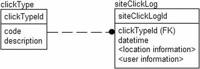
Figure 10-15. Sample foreign key relationship
Consider that you want to delete a clickType row that someone added inadvertently. Creating the row took several milliseconds. Deleting it shouldn’t take long at all, right? Well, even if there isn’t a single value in the table, if you don’t have an index on the foreign key in the siteClickLog table, it will take just over 10 seconds longer than eternity. Even though the value doesn’t exist in the table, the query processor would need to touch and check all five million rows for the value. From the statistics on the column, it can guess how many rows might exist, but it can’t definitively know that there is or is not a value because statistics are maintained asyncronously. (Ironically, because it is an existence search, it could fail on the first row it checked, but to successfully delete the row, every child row must be touched.)
However, if you have an index, deleting the row (or knowing that you can’t delete it) will take a very short period of time, because in the upper pages of the index, you’ll have all the unique values in the index, in this case, five values. There will be a fairly substantial set of leaf pages for the index, but only one page in each index level, usually no more than three or four pages, will need to be touched before the query processor can determine the existence of a row out of millions of rows. When NO ACTION is specified for the relationship, if just one row is found, the operation could be stopped. If you have cascading operations enabled for the relationship, the cascading options will need the index to find the rows to cascade to.
This adds more decisions when building indexes. Is the cost of building and maintaining the index during creation of millions of siteClickLog rows justified, or do you just bite the bullet and do deletes during off hours? Add a trigger such as the following, ignoring error handling in this example for brevity:
CREATE TRIGGER clickType$insteadOfDelete
ON clickType
INSTEAD OF DELETE
AS
INSERT INTO clickType_deleteQueue (clickTypeId)
SELECT clickTypeId
FROM inserted;
Then, you let your queries that return lists of clickType rows check this table when presenting rows to the users:
SELECT code, description, clickTypeId
FROM clickType
WHERE NOT EXISTS (SELECT *
FROM clickType_deleteQueue
WHERE clickType.clickTypeId =
clickType_deleteQueue.clickTypeId);
Now, assuming all code follows this pattern, the users will never see the value, so it won’t be an issue (at least not in terms of values being used; performance will suffer obviously). Then, you can delete the row in the wee hours of the morning without building the index. Whether or not an index proves useful generally depends on the purpose of the foreign key. I’ll mention specific types of foreign keys individually, each with their own signature usage:
- Domain tables: Used to implement a defined set of values and their descriptions
- Ownership: Used to implement a multivalued attribute of the parent
- Many-to-many resolution: Used to implement a many-to-many relationship physically
- One-to-one relationships: Cases where a parent may have only a single value in the related table
We’ll look at examples of these types and discuss when it’s appropriate to index them before the typical trial-and-error performance tuning, where the rule of thumb is to add indexes to make queries faster, while not slowing down other operations that create data.
In all cases, deleting the parent row requires a table scan of the child if there’s no index on the child row. This is an important consideration if there are deletes.
You use a domain table to enforce a domain using a table, rather than using a scalar value with a constraint. This is often done to enable a greater level of data about the domain value, such as a descriptive value. For example, consider the tables in Figure 10-16.
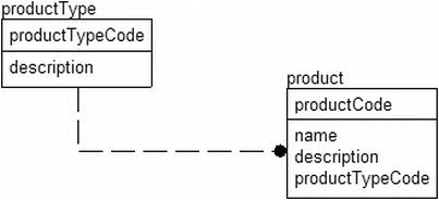
Figure 10-16. Sample domain table relationship
In this case, there are a small number of rows in the productType table. It’s unlikely that an index on the product.productTypeCode column would be of any value in a join, because you’ll generally be getting a productType row for every row you fetch from the product table.
What about the other direction, when you want to find all products of a single type? This can be useful if there aren’t many products, but in general, domain type tables don’t have enough unique values to merit an index. The general advice is that tables of this sort don’t need an index on the foreign key values, by default. Of course, deleting productType rows would need to scan the entire productType.
On the other hand, as discussed in the section introduction, sometimes an index can be useful when there are limited numbers of some value. For example, consider a user to userStatus relationship illustrated in Figure 10-17.
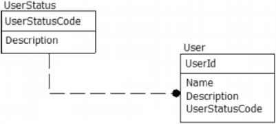
Figure 10-17. Sample domain table relationship with low cardinality
In this case, most users would be in the database with an active status. However, when a user was deactivated, you might need to do some action for that user. Since the number of inactive users would be far fewer than active users, it might be useful to have an index (possibly a filtered index) on the userStatusCode column for that purpose.
Some tables have no meaning without the existence of another table and pretty much exist to as part of another table (due to the way relational design works). When I am thinking about an ownership relationship, I am thinking of relationships that implement multivalued attributes for a row, just like an array in a procedural language does for an object. The main performance characteristic of this situation is that most of the time when the parent row is retrieved, the child rows are retrieved as well. You’ll be less likely to need to retrieve a child row and then look for the parent row.
For example, take the case of an invoice and its line items in Figure 10-18.
Figure 10-18. Sample ownership relationship
In this case, it’s essential to have an index on the invoiceLineItem.invoiceId column. Most access to the invoiceLineItem table results from a user’s need to get an invoice first. This situation is also ideal for an index because, usually, it will turn out to be a very selective index (unless you have large numbers of items and few sales).
Note that you should already have a UNIQUE constraint (and a unique index as a consequence of this) on the alternate key for the table—in this case, invoiceId and invoiceLineNumber. Therefore, you probably wouldn’t need to have an index on just invoiceId. What might be in question would be whether or not the index on invoiceId and invoiceLineNumber ought to be clustered. If you do most of your select operations using the invoiceId, this actually can be a good idea. However, you should be careful in this case because you can actually do a lot more fetches on the primary key value, since update and delete operations start out performing like a SELECT before the modification. For example, the application may end up doing one query to get the invoice line items and then update each row individually to do some operation. So always watch the activity in your database and tune accordingly.
Many-to-Many Resolution Table Relationships
When we have a many-to-many relationship, there certainly needs to be an index on the two migrated keys from the two parent tables. Think back to our Chapter 7 of games owned on a given platform (diagram repeated in Figure 10-19).
Figure 10-19. Sample many-to-many relationship
In this case, you should already have a unique index on gamePlatformId and gameId, and one of the two will necessarily be first in the composite index. If you need to search for both keys independently of one another, you may want to create an index on each column individually (or at least the column that is listed second in the uniqueness constraint’s index).
Take this example. If we usually look up a game by name (which would be alternate key indexed) and then get the platforms for this game, an index only on gameInstance.gameId would be much more useful and two-thirds the size of the alternate key index (assuming a clustering key of gameInstanceId).
One-to-one relationships generally require some form of unique index on the key in the parent table as well as on the migrated key in the child table. For example, consider the subclass example of a bankAccount, shown in Figure 10-20.
Figure 10-20. Sample one-to-one relationship
In this case, because these are one-to-one relationships, and there are already indexes on the primary key of each table, no other indexes would need to be added to effectively implement the relationship.
Indexing Views
I mentioned the use of persisted calculated columns in Chapter 6 for optimizing denormalizations for a single row, but sometimes, your denormalizations need to span multiple rows and include things like summarizations. In this section, I will introduce a way to take denormalization to the next level, using indexed views .
Indexing a view basically takes the virtual structure of the view and makes it a physical entity, albeit one managed completely by the query processor. The data to resolve queries with the view is generated as data is modified in the table, so access to the results from the view is just as fast as if it were an actual table. Indexed views give you the ability to build summary tables without any kind of manual operation or trigger; SQL Server automatically maintains the summary data for you. Creating indexed views is as easy as writing a query.
The benefits are twofold when using indexed views. First, when you use an indexed view directly in any edition of SQL Server, it does not have to do any calculations (editions less than Enterprise must specify NOEXPAND as a hint). Second, in the Enterprise Edition or greater (plus the Developer Edition), SQL Server automatically considers the use of an indexed view whenever you execute any query, even if the query doesn’t reference the view but the code you execute uses the same aggregates. SQL Server accomplishes this index view assumption by matching the executed query to each indexed view to see whether that view already has the answer to something you are asking for.
For example, we could create the following view on the product and sales tables in the Adventureworks2012 database. Note that only schema-bound views can be indexed as this makes certain that the tables and structures that the index is created upon won’t change underneath the view. (A more complete list of requirements is presented after the example.). Note that you actually have to be in the AdventureWorks2012 database, unlike other examples where I have addressed items to the database, because index views have strict requirements, which I will cover in more detail in the next section of this chapter.
USE AdventureWorks2012;
GO
CREATE VIEW Production.ProductAverageSales
WITH SCHEMABINDING
AS
SELECT Product.ProductNumber,
SUM(SalesOrderDetail.LineTotal) as TotalSales,
COUNT_BIG(*) as CountSales --must use COUNT_BIG for indexed view
FROM Production.Product as Product
JOIN Sales.SalesOrderDetail as SalesOrderDetail
ON Product.ProductID=SalesOrderDetail.ProductID
GROUP BY Product.ProductNumber;
This would do the calculations at execution time. We run the following query:
SELECT ProductNumber, TotalSales, CountSales
FROM Production.ProductAverageSales;
The plan looks like this:
|--Hash Match(Inner Join, HASH:([SalesOrderDetail].[ProductID])=
([Product].[ProductID]))
|--Hash Match(Aggregate, HASH:([SalesOrderDetail].[ProductID])
DEFINE:([Expr1004]=SUM([AdventureWorks2012].[Sales].
[SalesOrderDetail].[LineTotal] as
[SalesOrderDetail].[LineTotal]), [Expr1005]=COUNT(*)))
| |--Compute Scalar(DEFINE:([SalesOrderDetail].[LineTotal]=
[AdventureWorks2012].[Sales].[SalesOrderDetail].[LineTotal] as
[SalesOrderDetail].[LineTotal]))
| |--Compute Scalar(DEFINE:([SalesOrderDetail].[LineTotal]=
isnull((CONVERT_IMPLICIT(numeric(19,4),
[AdventureWorks2012].[Sales].[SalesOrderDetail].[UnitPrice] as
[SalesOrderDetail].[UnitPrice],0)*
((1.0)-CONVERT_IMPLICIT(numeric(19,4),
[AdventureWorks2012].[Sales].[SalesOrderDetail].
[UnitPriceDiscount] as [SalesOrderDetail].
[UnitPriceDiscount],0)))* CONVERT_IMPLICIT(numeric(5,0),
[AdventureWorks2012].[Sales].[SalesOrderDetail].[OrderQty]
as [SalesOrderDetail].[OrderQty],0),(0.000000))))
| |--Clustered Index
Scan(OBJECT:([AdventureWorks2012].[Sales].[SalesOrderDetail].
[PK_SalesOrderDetail_SalesOrderID_SalesOrderDetailID]
AS [SalesOrderDetail]))
|--Index Scan(OBJECT:(
[AdventureWorks2012].[Production].[Product].AK_Product_ProductNumber] AS [Product]))
This is a big plan for such a small query, for sure, and it’s hard to follow. It scans the SalesOrderDetail table, computes our scalar values, and then does a hash match aggregate and a hash match join to join the two sets together. For further reading on the join types, again consider a book in Kalen Delaney’s SQL Server Internals series.
This query executes pretty fast on my 1.8-GHz 8-GB laptop, but there’s a slight but noticeable delay. Say this query wasn’t fast enough, or it used too many resources to execute, and it is used extremely often. In this case, we might add an index on the view. Note that it is a clustered index, as the data pages will be ordered based on the key we chose. Consider your structure of the index just like you would on a physical table.
CREATE UNIQUE CLUSTERED INDEX XPKProductAverageSales on
Production.ProductAverageSales(ProductNumber);
SQL Server would then materialize the view and store it. Now, our queries to the view will be very fast. However, although we’ve avoided all the coding issues involved with storing summary data, we have to keep our data up to date. Every time data changes in the underlying tables, the index on the view changes its data, so there’s a performance hit in maintaining the index for the view. Hence, indexing views means that performance is great for reading but not necessarily for updating.
Now, run the query again:
SELECT ProductNumber, TotalSales, CountSales
FROM Production.ProductAverageSales;
The plan looks like the following:
|--Clustered Index Scan(OBJECT:(
[AdventureWorks2012].[Production].[ProductAverageSales].[XPKProductAverageSales]))
No big deal, right? We expected this result because we directly queried the view. On my test system, running the Developer Edition (which is functionally comparable to the Enterprise Edition), you get a great insight into how cool this feature is in the following query for getting the average sales per product:
SELECT Product.ProductNumber, SUM(SalesOrderDetail.LineTotal) / COUNT(*)
FROM Production.Product as Product
JOIN Sales.SalesOrderDetail as SalesOrderDetail
ON Product.ProductID=SalesOrderDetail.ProductID
GROUP BY Product.ProductNumber;
We’d expect the plan for this query to be the same as the first query of the view was, because we haven’t referenced anything other than the base tables, right? I already told you the answer, so here’s the plan:
| -- Compute
Scalar(DEFINE:(
[Expr1006]=[AdventureWorks2012].[Production].ProductAverageSales].
[totalSales]/CONVERT_IMPLICIT(numeric(10,0),[Expr1005],0)))
|--Compute Scalar(DEFINE:([Expr1005]=
CONVERT_IMPLICIT(int,[AdventureWorks2012].[Production].
[ProductAverageSales].[averageTotal],0)))
|--Clustered Index
Scan(OBJECT:([AdventureWorks2012].[Production].[ProductAverageSales].
[XPKProductAverageSales]))
There are two scalar computes—one for the division and one to convert the bigint from the COUNT_BIG(*) to an integer—and the other to scan through the indexed view’s clustered index. You will notice that the plan references the ProductAverageSales indexed view, and we did not reference it directly in our query. The ability to use the optimizations from an indexed view indirectly is a neat feature that allows you to build in some guesses as to what ad hoc users will be doing with the data and giving them performance they didn’t even ask for.
![]() Tip The indexed view feature in the Enterprise Edition and greater can also come in handy for tuning third-party systems that work on an API that is not tunable in a direct manner (that is, to change the text of a query to make it more efficient).
Tip The indexed view feature in the Enterprise Edition and greater can also come in handy for tuning third-party systems that work on an API that is not tunable in a direct manner (that is, to change the text of a query to make it more efficient).
There are some pretty heavy caveats, though. The restrictions on what can be used in a view, prior to it being indexed, are fairly tight. The most important things that cannot be done are as follows:
- Use the SELECT * syntax—columns must be explicitly named.
- Use a CLR user defined aggregate.
- Use UNION, EXCEPT, or INTERSECT in the view.
- Use any subqueries.
- Use any outer joins or recursively join back to the same table.
- Specify TOP in the SELECT clause.
- Use DISTINCT.
- Include a SUM() function if it references more than one column.
- Use COUNT(*), though COUNT_BIG(*) is allowed.
- Use almost any aggregate function against a nullable expression.
- Reference any other views, or use CTEs or derived tables.
- Reference any nondeterministic functions.
- Reference data outside the database.
- Reference tables owned by a different owner.
And this isn’t all. You must meet several pages of requirements, documented in SQL Server Books Online in the section “Creating Indexed Views.” However, these are the most significant ones that you need to consider before using indexed views.
Although this might all seem pretty restrictive, there are good reasons for all these rules. Maintaining the indexed view is analogous to writing our own denormalized data maintenance functions. Simply put, the more complex the query to build the denormalized data, the greater the complexity in maintaining it. Adding one row to the base table might cause the view to need to recalculate, touching thousands of rows.
Indexed views are particularly useful when you have a view that’s costly to run, but the data on which it’s based doesn’t change a tremendous amount. As an example, consider a decision-support system where you load data once a day. There’s overhead either maintaining the index, or possibly just rebuilding it, but if you can build the index during off hours, you can omit the cost of redoing joins and calculations for every view usage.
![]() Tip With all the caveats, indexed views can prove useless for some circumstances. An alternative method is to materialize the results of the data by inserting the data into a permanent table. For example, for our sample query, we’d create a table with three columns (productNumber, totalSales, and countSales), and then we’d do an INSERT
INTO
ProductAverageSales
SELECT . . . . We’d put the results of the query in this table. Any query works here, not just one that meets the strict guidelines. It doesn’t help out users making ad hoc queries who don’t directly query the data in the table, but it certainly improves performance of queries that directly access the data, particularly if perfect results are not needed, since data will usually be a little bit old due to the time required to refresh the data.
Tip With all the caveats, indexed views can prove useless for some circumstances. An alternative method is to materialize the results of the data by inserting the data into a permanent table. For example, for our sample query, we’d create a table with three columns (productNumber, totalSales, and countSales), and then we’d do an INSERT
INTO
ProductAverageSales
SELECT . . . . We’d put the results of the query in this table. Any query works here, not just one that meets the strict guidelines. It doesn’t help out users making ad hoc queries who don’t directly query the data in the table, but it certainly improves performance of queries that directly access the data, particularly if perfect results are not needed, since data will usually be a little bit old due to the time required to refresh the data.
Index Dynamic Management View Queries
In this section, I want to provide a couple of queries that use the dynamic management views that you may find handy when you are tuning your system or index usage. In SQL Server 2005, Microsoft added a set of objects (views and table-valued functions) to SQL Server that gave us access to some of the deep metadata about the performance of the system. A great many of these objects are useful for managing and tuning SQL Server, and I would suggest you do some reading about these objects (not to be overly self serving, but the book Performance Tuning with SQL Server Dynamic Management Views (High Performance Sql Server) by Tim Ford and myself published by Simple-Talk is my favorite book on the subject!). I do want to provide you with some queries that will likely be quite useful for you when doing any tuning using indexes.
The first query we’ll discuss will provide you a peek at what indexes the optimizer thought might be useful. It can be very helpful when tuning a database, particularly a very busy databsase executing thousands of queries a minute. I have personally used it to tune third-party systems where I didn’t have a lot of access to the queries in the system and using profiler was simply far too cumbersome with too many queries to effectively tune manually.
It uses three of the dynamic management views that are part of the missing index family of objects. These are:
- sys.dm_db_missing_index_groups: This relates missing index groups with the indexes in the group. There is only one index to a group, as of the 2011 release.
- sys.dm_db_missing_index_group_stats: This provides statistics of how much the indexes in the group (only one in 2005; see the previous section) would have helped (and hurt) the system.
- sys.dm_db_missing_index_details: This provides information about the index that the optimizer would have chosen to have available.
The query is as follows. I won’t attempt to build a scenario where you can test this functionality out in this book, but run the query on one of your development servers and check the results. The results will likely make you want to run it on your production server:
SELECT ddmid.statement AS object_name, ddmid.equality_columns, ddmid.inequality_columns,
ddmid.included_columns, ddmigs.user_seeks, ddmigs.user_scans,
ddmigs.last_user_seek, ddmigs.last_user_scan, ddmigs.avg_total_user_cost,
ddmigs.avg_user_impact, ddmigs.unique_compiles
FROM sys.dm_db_missing_index_groups as ddmig
JOIN sys.dm_db_missing_index_group_stats as ddmigs
ON ddmig.index_group_handle = ddmigs.group_handle
JOIN sys.dm_db_missing_index_details as ddmid
ON ddmid.index_handle = ddmig.index_handle
ORDER BY ((user_seeks + user_scans) * avg_total_user_cost * (avg_user_impact * 0.01)) DESC;
The query returns the following information about the structure of the index that might have been useful:
- object_name: This is the database and schema qualified object name of the object that the index would have been useful on. The data returned is for all databases on the entire server
- equality_columns: These are the columns that would have been useful, based on an equality predicate. The columns are returned in a comma-delimited list.
- inequality_columns: These are the columns that would have been useful, based on an inequality predicate (which as we have discussed is any comparison other than column = value or column in (value, value1)).
- included_columns: These columns, if added to the index via an INCLUDE clause, would have been useful to cover the query results and avoid a key lookup operation in the plan.
As discussed earlier, the equality columns would generally go first in the index column definition, but it isn’t guaranteed that that will make the correct index. These are just guidelines, and using the next DMV query I will present, you can discover if the index you create turns out to be of any value.
- unique_compiles: The number of plans that have been compiled that might have used the index
- user_seeks: The number of seek operations in user queries might have used the index
- user_scans: The number of scan operations in user queries that might have used the index
- last_user_seek: The last time that a seek operation might have used the index
- last_user_scan: The last time that a scan operation might have used the index
- avg_total_user_cost: Average cost of queries that could have been helped by the group of indexes
- avg_user_impact: The percentage of change in cost that the index is estimated to make for user queries
Note that I sorted the query results as (user_seeks + user_scans) * avg_total_user_cost * (avg_user_impact * 0.01) based on the initial blog I read using the missing indexes, “Fun for the Day” – Automated Auto-Indexing ( http://blogs.msdn.com/queryoptteam/archive/2006/06/01/613516.aspx ). I generally use some variant of that to determine what is most important. For example, I might use order by (user_seeks + user_scans) to see what would have been useful the most times. It really just depends on what I am trying to scan; with all such queries, it pays to try out the query and see what works for your situation.
To use the output, you can create a CREATE INDEX statement from the values in the four structural columns. Say you received the following results:
| object_name | equality_columns | inequality_columns |
| ------------- | ------------- | ------------- |
| databasename.schemaname.tablename | columnfirst, columnsecond | columnthird |
included_columns
-------------------------
columnfourth, columnfififth
You could build the following index to satisfy the need:
CREATE INDEX XName ON databaseName.schemaName.TableName(columnfirst, columnsecond, columnthird) INCLUDE (columnfourth, columnfififth);
Next, see if it helps out performance in the way you believed it might. And even if you aren’t sure of how the index might be useful, create it and just see if it has an impact.
Books Online lists the following limitations to consider:
- It is not intended to fine-tune an indexing configuration.
- It cannot gather statistics for more than 500 missing index groups.
- It does not specify an order for columns to be used in an index.
- For queries involving only inequality predicates, it returns less accurate cost information.
- It reports only include columns for some queries, so index key columns must be manually selected.
- It returns only raw information about columns on which indexes might be missing. This means the information returned may not be sufficient by itself without additional processing before building the index.
- It does not suggest filtered indexes.
- It can return different costs for the same missing index group that appears multiple times in XML showplans.
- It does not consider trivial query plans.
Probably the biggest concern is that it can specify a lot of overlapping indexes, particularly when it comes to included columns, since each entry could have been specifically created for distinct queries. For very busy systems, you may find a lot of the suggestions include very large sets of include columns that you may not want to implement.
However, limitations aside, the missing index dynamic management view are amazingly useful to help you see places where the optimizer would have liked to have an index and one didn’t exist. This can greatly help diagnose very complex performance/indexing concerns, particularly ones that need a large amount of INCLUDE columns to cover complex queries. This feature is turned on by default and can only be disabled by starting SQL Server with a command line parameter of –x. This will, however, disable keeping several other statistics like CPU time and cache-hit ratio stats.
Using this feature and the query in the next section that can tell you what indexes have been used, you can use these index suggestions in an experimental fashion, just building a few of the indexes and see if they are used and what impact they have on your performance tuning efforts.
The second query gives statistics on how an index has been used to resolve queries. Most importantly, it tells you the number of times a query was used to find a single row (user_seeks), a range of values, or to resolve a non-unique query (user_scans), if it has been used to resolve a bookmark lookup (user_lookups), and how many changes to the index (user_updates). If you want deeper information on how the index was modified, check sys.dm_db_index_operational_stats). The query makes use of the sys.dm_db_index_usage_stats object that provides just what the names says, usage statistics:
SELECT OBJECT_SCHEMA_NAME(indexes.object_id) + '.' +
OBJECT_NAME(indexes.object_id) as objectName,
indexes.name,
CASE WHEN is_unique = 1 then 'UNIQUE '
else '' END + indexes.type_desc as index_type,
ddius.user_seeks, ddius.user_scans, ddius.user_lookups,
ddius.user_updates, last_user_lookup, last_user_scan, last_user_seek,last_user_update
FROM sys.indexes
LEFT OUTER JOIN sys.dm_db_index_usage_stats as ddius
ON indexes.object_id = ddius.object_id
AND indexes.index_id = ddius.index_id
AND ddius.database_id = db_id()
ORDER BY ddius.user_seeks + ddius.user_scans + ddius.user_lookups DESC;
The query (as written) is database dependent in order to look up the name of the index in sys.indexes, which is a database-level catalog view. The sys.dm_db_index_usage_stats object returns all indexes (including heaps and the clustered index) from the entire server (there will not be a row for sys.dm_db_index_usage_stats unless the index has been used since the last time the server has been started). The query will return all indexes for the current database (since the DMV is filtered on db_id() in the join criteria) and will return:
- object_name: Schema-qualified name of the table.
- index_name: The name of the index (or table) from sys.indexes.
- index_type: The type of index, including uniqueness and clustered/nonclustered.
- user_seeks: The number of times the index has been used in a user query in a seek operation (one specific row).
- user_scans: The number of times the index has been used by scanning the leaf pages of the index for data.
- user_lookups: For clustered indexes only, this is the number of times the index has been used in a bookmark lookup to fetch the full row. This is because nonclustered indexes use the clustered indexes key as the pointer to the base row.
- user_updates: The number of times the index has been modified due to a change in the table’s data.
- last_user_seek: The date and time of the last user seek operation.
- last_user_scan: The date and time of the last user scan operation.
- last_user_lookup: The date and time of the last user lookup operation.
- last_user_update: The date and time of the last user update operation.
There are also columns for system utilizations of the index in operations such as automatic statistics operations: system_seeks, system_scans, system_lookups, system_updates, last_system_seek, last_system_scan, last_system_lookup, and last_system_update.
This is one of the most interesting views that I often use in performance tuning. It gives you the ability to tell when indexes are not being used. It is easy to see when an index is being used by a query by simply looking at the plan. But now, using this dynamic management view, you can see over time what indexes are used, not used, and probably more importantly, updated many, many times without ever being used.
One of the biggest tasks for the DBA of a system is to make sure that the structures of indexes and tables are within a reasonable tolerance. You can decide whether to reorganize or to rebuild using the criteria stated by SQL Server Books Online in the topic for the dynamic management view sys.dm_db_index_physical_stats. You can check the FragPercent column and REBUILD indexes with greater than 30% fragmentation and REORGANIZE those that are just lightly fragmented.
SELECT s.[name] AS SchemaName,
o.[name] AS TableName,
i.[name] AS IndexName,
f.[avg_fragmentation_in_percent] AS FragPercent,
f.fragment_count ,
f.forwarded_record_count --heap only
FROM sys.dm_db_index_physical_stats(DB_ID(), NULL, NULL, NULL, DEFAULT) f
JOIN sys.indexes as i
ON f.[object_id] = i.[object_id] AND f.[index_id] = i.[index_id]
JOIN sys.objects as o
ON i.[object_id] = o.[object_id]
JOIN sys.schemas as s
ON o.[schema_id] = s.[schema_id]
WHERE o.[is_ms_shipped] = 0
AND i.[is_disabled] = 0; -- skip disabled indexes
sys.dm_db_index_physical_stats will give you a lot more information about the internal physical structures of your tables and indexes than I am making use of here. If you find you are having a lot of fragmentation, adjusting the fill factor of your tables or indexes (specified as a percentage of page size to leave empty for new rows) in CREATE INDEX and PRIMARY KEY and UNIQUEconstraint CREATE/ALTER DDL statements can help tremendously. How much space to leave will largely depend on your exact situation, but minimally, you want to leave approximately enough space for one full additional row to be added to each page.
Best Practices
Indexing is a complex subject, and even though this is not a short chapter, we’ve only scratched the surface. The following best practices are what I use as a rule of thumb when creating a new database solution. Note that I assume that you’ve applied UNIQUE constraints in all places where they make logical sense. These constraints most likely should be there, even if they slow down your application (there are exceptions, but if a set of values needs to be unique, it needs to be unique). From there, it’s all a big tradeoff. The first rule is the most important.
- There are few reasons to add indexes to tables without testing: Add nonconstraint indexes to your tables only as needed to enhance performance. In many cases, it will turn out that no index is needed to achieve decent performance. A caveat can be foreign key indexes.
- Choose clustered index keys wisely: All nonclustered indexes will use the clustering key as their row locator, so the performance of the clustered index will affect all other index utilization. If the clustered index is not extremely useful, it can affect the other indexes as well.
- Keep indexes as thin as possible: Only index the columns that are selective enough in the main part of the index. Use the INCLUDE clause on the CREATE INDEX statement if you want to include columns only to cover the data used by a query.
- Consider several thin indexes rather than one monolithic index: SQL Server can use multiple indexes in a query efficiently. This can be a good tool to support ad hoc access where the users can choose between multiple situations.
- Be careful of the cost of adding an index: When you insert, update, or delete rows from a table with an index, there’s a definite cost to maintaining the index. New data added might require page splits, and inserts, updates, and deletes can cause a reshuffling of the index pages.
- Carefully consider foreign key indexes: If child rows are selected because of a parent row (including on a foreign key checking for children on a delete operation), an index on the columns in a foreign key is generally a good idea.
- UNIQUE constraints are used to enforce uniqueness, not unique indexes: Unique indexes are used to enhance performance by telling the optimizer that an index will only return one row in equality comparisons. Users shouldn’t get error messages from a unique index violation.
- Experiment with indexes to find the combination that gives the most benefit: Using the missing index and index usage statistics dynamic management views, you can see what indexes the optimizer needed or try your own, and then see if your choices were ever used by the queries that have been executed.
Apply indexes during your design in a targeted fashion, making sure not to overdesign for performance too early in the process. The normalization pattern is built to give great performance as long as you design for the needs of the users of the system, rather than in an academic manner taking things to the extreme that no one will ever use. The steps we have covered through this book for proper indexing are:
- Apply all the UNIQUE constraints that need to be added to enforce necessary uniqueness for the integrity of the data (even if the indexes are never used for performance, though generally they will).
- Minimally, index all foreign key constraints where the parent table is likely to be the driving force behind fetching rows in the child (such as invoice to invoice line item).
- Start performance testing, running load tests to see how things perform.
- Identify queries that are slow, and consider the following:
- Add indexes using any tools you have at your disposal.
- Eliminate clustered index row lookups by covering queries, possibly using the INCLUDE keyword on indexes.
- Materialize query results, either by indexed view or by putting results into permanent tables.
- Work on data location strategies with filegroups, partitioning, and so on.
- Consider compression if you are using Enterprise or Data Center edition to lower the amount of data that is stored on disk.
Summary
In the first nine chapters of this book, we worked largely as if the relational engine was magical like the hat that brought Frosty to life and that the engine could do almost anything as long as we followed the basic relational principals. Magic, however, is almost always an illusion facilitated by the hard work of someone trying to let you see only what you want to see. In this chapter, we left the world of relational programming and took a peak under the covers to see what makes the magic work, which turns out to be lots and lots of code that has been evolving for the past 16 plus years (just counting from the major rewrite of SQL Server in version 7.0.) Much of the T-SQL code written for version 1.0 would work today, and almost all of it would run with a little bit of translation, yet probably none of the engine code from 1.0 persists today.
This is one of the reasons why, in this book on design, my goals for this chapter are not to make you an expert on the internals of SQL Server but rather to give you an overview of how SQL Server works enough to help guide your designs and understand the basics of performance.
We looked at the physical structure of how SQL Server stores data, which is separate from the database-schema-table-column model that is natural in the relational model. Physically speaking, for normal row data, database files are the base container. Files are grouped into filegroups, and filegroups are owned by databases. You can get some control over SQL Server I/O by where you place the files.
Inside files, data is managed in extents of 64KB and then is broken up into 8-KB pages. Almost all I/O is performed in these sizes. Pages that are used in the same object are generally linked to one another to facilitate scanning. Pages are the building blocks that are used to hold all of the data and indexes that we take for granted when we write SELECT * FROM TABLE and all that wonderful code that has been written to translate that simple statement into a set of results starts churning to produce results quickly and correctly. How the data is actually formatted on page is based on a lot of factors: compression, partitioning, and most of all, indexing.
Indexing, like the entire gamut of performance-tuning topics, is hard to cover with any specificity on a written page (particularly not as a chapter of a larger book on design), I’ve given you some information about the mechanics of tables and indexes, and a few best practices, but to be realistic, it’s never going to be enough without you working with a realistic, active working test system.
Tuning with indexes requires a lot of basic knowledge about structures and utilization of those structures applied on a large scale. Joins decide whether or not to use an index based on many factors, and the indexes available to a query affect the join operators chosen. The best teacher for this is the school of “having to wait for a five-hour query to process.” Most people, when starting out, begin on small systems; they code any way they want and slap indexes on everything, and it works great. SQL Server has a very advanced optimizer that covers a multitude of such sins, particularly on a low-concurrency, low-usage system. As your system grows and requires more and more resources, it becomes more and more difficult to do performance tuning haphazardly, and all too often, programmers start applying indexes without actually seeing what effect they will have on the overall performance.
Designing physical structures is an important step to building high-performance systems that must be done during multiple phases of the project, starting when you are still modeling, and only being completed with performance testing, and honestly, continuing into production operation.
In the next chapter, we will talk a bit more about hardware as we look at some of the concerns for building highly concurrent systems with many users executing simultaneously. Having moderate- to high-level server-class hardware with fast RAID arrays and multiple channels to the disk storage, you can spread the data out over multiple filegroups, as I discussed in the basic table structure section earlier.