
![]()
I like rhyme because it is memorable; I like form because having to work to a pattern gives me original ideas.
—Anne Stevenson
There is an old saying that you shouldn’t try to reinvent the wheel, and honestly, in essence it is a very good saying. But with all such sayings, a modicum of common sense is required for its application. If everyone down through history took the saying literally, your car would have wheels made out of the trunk of a tree (which the Mythbusters proved you could do in their “Good Wood” episode), since that clearly could have been one of the first wheel-like machines that was used. If everyone down through history had said “that’s good enough,” driving to Wally World in the family truckster would be a far less comfortable experience.
Over time, however, the basic concept of a wheel has been intact, from rock wheel, to wagon wheel, to steel-belted radials, and even a wheel of cheddar. Each of these is round, able to move itself, and other stuff, by rolling from place A to place B. Each solution follows that common pattern but diverges to solve a particular problem. The goal of a software programmer should be to first try understanding existing techniques and then either use or improve them. Solving the same problem over and over without any knowledge of the past is nuts.
Of course, in as much as there are positive patterns that work, there are also negative patterns that have failed over and over down through history. Take personal flight. For many, many years, truly intelligent people tried over and over to strap wings on their arms or backs and fly. They were close in concept, but just doing the same thing over and over was truly folly. Once it was understood how to apply Bernoulli’s principle to building wings and what it would truly take to fly, the Wright Brothers applied this principal, plus principles of lift, to produce the first flying machine. If you ever happen by Kitty Hawk, NC, you can see the plane and location of that flight. Not an amazing amount has changed between that airplane and today’s airplanes in basic principle. Once they got it right, it worked.
In designing and implementing a database, you get the very same sort of things going on. The problem with patterns and anti-patterns is that you don’t want to squash new ideas immediately. The anti-patterns I will present later in this chapter may be very close to something that becomes a great pattern. Each pattern is there to solve a problem, and in some cases, the problem solved isn’t worth the side effects.
Throughout this book so far, we have covered the basic implementation tools that you can use to assemble solutions that meet your real-world needs. In this chapter, I am going to extend this notion and present a few deeper examples where we assemble a part of a database that deals with common problems that show up in almost any database solution. The chapter will be broken up into two major sections. In the first section, we will cover patterns that are common and generally desirable to use. The second half will be anti-patterns, or patterns that you may frequently see that are not desirable to use (along with the preferred method of solution, naturally).
Desirable Patterns
In this section, I am going to cover a good variety of implementation patterns that can be used to solve a number of very common problems that you will frequently encounter. By no means should this be confused with a comprehensive list of the types of problems you may face; think of it instead as a sampling of methods of solving some common problems.
The patterns and solutions that I will present are as follows:
- Uniqueness : Moving beyond the simple uniqueness we covered in the first chapters of this book, we’ll look at some very realistic patterns of solutions that cannot be implemented with a simple uniqueness constraint.
- Data-driven design : The goal of data driven design is that you never hard-code values that don’t have a fixed meaning. You break down your programming needs into situations that can be based on sets of data values that can be modified without affecting code.
- Hierarchies : A very common need is to implement hierarchies in your data. The most common example is the manager-employee relationship. In this section, I will demonstrate the two simplest methods of implementation and introduce other methods that you can explore.
- Images, documents, and other files : There is, quite often, a need to store documents in the database, like a web users’ avatar picture, or a security photo to identify an employee, or even documents of many types. We will look at some of the methods available to you in SQL Server and discuss the reasons you might choose one method or another.
- Generalization : In this section, we will look at some ways that you will need to be careful with how specific you make your tables so that you fit the solution to the needs of the user.
- Storing user-specified data : You can’t always design a database to cover every known future need. In this section, I will cover some of the possibilities for letting users extend their database themselves in a manner that can be somewhat controlled by the administrators.
![]() Note I am always looking for other patterns that can solve common issues and enhance your designs (as well as mine). On my web site (drsql.org), I may make additional entries available over time, and please leave me comments if you have ideas for more.
Note I am always looking for other patterns that can solve common issues and enhance your designs (as well as mine). On my web site (drsql.org), I may make additional entries available over time, and please leave me comments if you have ideas for more.
If you have been reading this book straight through, you’re probably getting a bit sick of hearing about uniqueness. The fact is, uniqueness is one of the largest problems you will tackle when designing a database, because telling two rows apart from one another can be a very difficult task. Most of our efforts so far have been in trying to tell two rows apart, and that is still a very important task that you always need to do.
But, in this section, we will explore a few more types of uniqueness that hit at the heart of the problems you will come across:
- Selective: Sometimes, we won’t have all of the information for all rows, but the rows where we do have data need to be unique. As an example, consider the driver’s license numbers of employees. No two people can have the same information, but not everyone will necessarily have one.
- Bulk : Sometimes, we need to inventory items where some of the items are equivalent. For example, cans of corn in the grocery store. You can’t tell each item apart, but you do need to know how many you have.
- Range: In this case, we want to make sure that ranges of data don’t overlap, like appointments. For example, take a hair salon. You don’t want Mrs. McGillicutty to have an appointment at the same time as Mrs. Mertz, or no one is going to end up happy.
- Approximate: The most difficult case is the most common, in that it can be really difficult to tell two people apart who come to your company for service. Did two Louis Davidsons purchased toy airplanes yesterday? Possibly at the same phone number and address? Probably not, though you can’t be completely sure without asking.
Uniqueness is one of the biggest struggles in day-to-day operations, particularly in running a company, as it is sometimes difficult to get customers to divulge identifying information, particularly when they’re just browsing. But it is the most important challenge to identify and coalesce unique information so we don’t end up with the ten employees with the same SSN numbers, far fewer cans of corn than we expected, ten appointments at the same time, or so we don’t send out 12 flyers to the same customer because we didn’t get that person uniquely identified.
We previously discussed PRIMARY KEY and UNIQUE constraints, but in some situations, neither of these will exactly fit the situation. For example, you may need to make sure some subset of the data, rather than every row, is unique. An example of this is a one-to-one relationship where you need to allow nulls, for example, a customerSettings table that lets you add a row for optional settings for a customer. If a user has settings, a row is created, but you want to ensure that only one row is created.
For example, say you have an employee table, and each employee can possibly have an insurance policy. The policy numbers must be unique, but the user might not have a policy.
There are two solutions to this problem that are common:
- Filtered indexes : This feature that was new in SQL Server 2008. The CREATE INDEX command syntax has a WHERE clause so that the index pertains only to certain rows in the table.
- Indexed view : In recent versions prior to 2008, the way to implement this is to create a view that has a WHERE clause and then index the view.
As a demonstration, I will create a schema and table for the human resources employee table with a column for employee number and insurance policy number as well (the examples in this chapter will be placed in a file named Chapter8 in the downloads and hence, any error messages will appear there as well).
CREATE SCHEMA HumanResources;
GO
CREATE TABLE HumanResources.employee
(
EmployeeId int NOT NULL IDENTITY(1,1) CONSTRAINT PKalt_employee PRIMARY KEY,
EmployeeNumber char(5) not null
CONSTRAINT AKalt_employee_employeeNummer UNIQUE,
--skipping other columns you would likely have
InsurancePolicyNumber char(10) NULL
);
One of the lesser known but pretty interesting features of indexes is the filtered index . Everything about the index is the same, save for the WHERE clause. So, you add an index like this:
--Filtered Alternate Key (AKF)
CREATE UNIQUE INDEX AKFHumanResources_Employee_InsurancePolicyNumber ON
HumanResources.employee(InsurancePolicyNumber)
WHERE InsurancePolicyNumber IS NOT NULL;
Then, create an initial sample row :
INSERT INTO HumanResources.Employee (EmployeeNumber, InsurancePolicyNumber)
VALUES ('A0001','1111111111'),
If you attempt to give another employee the same insurancePolicyNumber
INSERT INTO HumanResources.Employee (EmployeeNumber, InsurancePolicyNumber)
VALUES ('A0002','1111111111'),
this fails:
Msg 2601, Level 14, State 1, Line 1
Cannot insert duplicate key row in object 'HumanResources.employee' with unique index 'AKFHumanResources_Employee_InsurancePolicyNumber'. The duplicate key value is (1111111111).
However, adding two rows with null will work fine:
INSERT INTO HumanResources.Employee (EmployeeNumber, InsurancePolicyNumber)
VALUES('A0003','2222222222'),
('A0004',NULL),
('A0005',NULL);
You can see that this:
SELECT *
FROM HumanResources.Employee;
returns the following:
| EmployeeId0 | EmployeeNumber | InsurancePolicyNumber |
| ------------------ | ------------------------- | ----------------------------------- |
| 1 | A0001 | 1111111111 |
| 3 | A0003 | 2222222222 |
| 4 | A0004 | NULL |
| 5 | A0005 | NULL |
The NULL example is the classic example, because it is common to desire this functionality. However, this technique can be used for more than just NULL exclusion. As another example, consider the case where you want to ensure that only a single row is set as primary for a group of rows, such as a primary contact for an account:
CREATE SCHEMA Account;
GO
CREATE TABLE Account.Contact
(
ContactId varchar(10) not null,
AccountNumber char(5) not null, --would be FK in full example
PrimaryContactFlag bit not null,
CONSTRAINT PKalt_accountContact
PRIMARY KEY(ContactId, AccountNumber)
);
Again, create an index, but this time, choose only those rows with primaryContactFlag = 1. The other values in the table could have as many other values as you want (of course, in this case, since it is a bit, the values could be only 0 or 1):
CREATE UNIQUE INDEX
AKFAccount_Contact_PrimaryContact
ON Account.Contact(AccountNumber)
WHERE PrimaryContactFlag = 1;
If you try to insert two rows that are primary, as in the following statements that will set both contacts 'fred' and 'bob' as the primary contact for the account with account number '11111':
INSERT INTO Account.Contact
SELECT 'bob','11111',1;
GO
INSERT INTO Account.Contact
SELECT 'fred','11111',1;
the following error is returned:
Msg 2601, Level 14, State 1, Line 1
Cannot insert duplicate key row in object 'Account.Contact' with unique index 'AKFAccount_Contact_PrimaryContact'. The duplicate key value is (11111).
To insert the row with 'fred' as the name and set it as primary (assuming the 'bob' row was inserted previously), you will need to update the other row to be not primary and then insert the new primary row:
BEGIN TRANSACTION;
UPDATE Account.Contact
SET primaryContactFlag = 0
WHERE accountNumber = '11111';
INSERT Account.Contact
SELECT 'fred','11111', 1;
COMMIT TRANSACTION;
Note that in cases like this you would definitely want to use a transaction in your code so you don’t end up without a primary contact if the insert fails for some other reason.
Prior to SQL Server 2008, where there were no filtered indexes, the preferred method of implementing this was to create an indexed view. There are a couple of other ways to do this (such as in a trigger or stored procedure using an EXISTS query , or even using a user-defined function in a CHECK constraint), but the indexed view is the easiest. Then when the insert does its cascade operation to the indexed view, if there are duplicate values, the operation will fail. You can use indexed views in all versions of SQL Server, though only Enterprise Edition will make special use of the indexes for performance purposes. (In other versions, you have to specifically reference the indexed view to realize performance gains. Using indexed views for performance reasons will be demonstrated in Chapter 10.)
Returning to the InsurancePolicyNumber uniqueness example, you can create a view that returns all rows other than null insurancePolicyNumber values. Note that it has to be schema bound to allow for indexing:
CREATE VIEW HumanResources.Employee_InsurancePolicyNumberUniqueness
WITH SCHEMABINDING
AS
SELECT InsurancePolicyNumber
FROM HumanResources.Employee
WHERE InsurancePolicyNumber IS NOT NULL;
Now, you can index the view by creating a unique, clustered index on the view:
CREATE UNIQUE CLUSTERED INDEX
AKHumanResources_Employee_InsurancePolicyNumberUniqueness
ON HumanResources.Employee_InsurancePolicyNumberUniqueness(InsurancePolicyNumber);
Now, attempts to insert duplicate values will be met with the following (assuming you drop the existing filtered index, which will be included in the code download.)
Msg 2601, Level 14, State 1, Line 1
Cannot insert duplicate key row in object 'HumanResources.
Employee_InsurancePolicyNumberUniqueness' with unique index
'AKHumanResources_Employee_InsurancePolicyNumberUniqueness'.
The duplicate key value is (1111111111).
The statement has been terminated.
Both of these techniques are really quite fast and easy to implement. However, the filtered index has a greater chance of being useful for searches against the table, so it is really just a question of education for the programming staff members who might come up against the slightly confusing error messages in their UI or SSIS packages, for example (even with good naming I find I frequently have to look up what the constraint actually does when it makes one of my SSIS packages fail). Pretty much no constraint error should be bubbled up to the end users, unless they are a very advanced group of users, so the UI should be smart enough to either prevent the error from occurring or at least translate it into words that the end user can understand.
Sometimes, we need to inventory items where some of the items are equivalent, for example, cans of corn in the grocery store. You can’t even tell them apart by looking at them (unless they have different expiration dates, perhaps), but it is a very common need to know how many you have. Implementing a solution that has a row for every canned good in a corner market would require a very large database even for a very small store, and as you sold each item, you would have to allocate those rows as they were sold. This would be really quite complicated and would require a heck of a lot of rows and data manipulation . It would, in fact, make some queries easier, but it would make data storage a lot more difficult.
Instead of having one row for each individual item, you can implement a row per type of item. This type would be used to store inventory and utilization , which would then be balanced against one another. In Figure 8-1, I show a very simplified model of such activity:
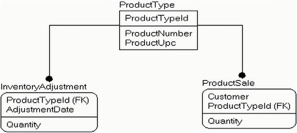
Figure 8-1. Simplified Inventory Model
In the InventoryAdjustment table , you would record shipments coming in, items stolen, changes to inventory after taking inventory (could be more or less, depending on the quality of the data you had), and in the product sale table (probably a sales or invoicing table in a complete model), you record when product is removed from inventory for a good reason.
The sum of the InventoryAdjustment Quantity less the ProductSale Quantity should be 0 or greater and should tell you the amount of product on hand. In the more realistic case, you would have a lot of complexity for backorders, future orders, returns, and so on, but the concept is basically the same. Instead of each row representing a single item, it represents a handful of items.
The following miniature design is an example I charge students with when I give my day-long seminar on database design. It is referencing a collection of toys, many of which are exactly alike:
A certain person was obsessed with his Lego® collection . He had thousands of them and wanted to catalog his Legos both in storage and in creations where they were currently located and/or used. Legos are either in the storage “pile” or used in a set. Sets can either be purchased, which will be identified by an up to five-digit numeric code, or personal, which have no numeric code. Both styles of set should have a name assigned and a place for descriptive notes.
Legos come in many shapes and sizes, with most measured in 2 or 3 dimensions. First in width and length based on the number of studs on the top, and then sometimes based on a standard height (for example, bricks have height; plates are fixed at 1/3 of 1 brick height unit). Each part comes in many different standard colors as well. Beyond sized pieces, there are many different accessories (some with length/width values), instructions, and so on that can be catalogued.
Example pieces and sets are shown in Figure 8-2.
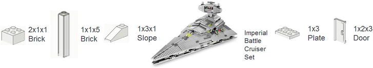
Figure 8-2. Sample Lego® parts for a database
To solve this problem, I will create a table for each type of set of Legos that are owned (which I will call Build, since “set” is a bad word for a SQL name, and “build” actually is better anyhow to encompass a personal creation):
CREATE SCHEMA Lego;
GO
CREATE TABLE Lego.Build
(
BuildId int NOT NULL CONSTRAINT PKLegoBuild PRIMARY KEY,
Name varchar(30) NOT NULL CONSTRAINT AKLegoBuild_Name UNIQUE,
LegoCode varchar(5) NULL, --five character set number
InstructionsURL varchar(255) NULL --where you can get the PDF of the instructions
);
Then, add a table for each individual instances of that build, which I will call BuildInstance :
CREATE TABLE Lego.BuildInstance
(
BuildInstanceId Int NOT NULL CONSTRAINT PKLegoBuildInstance PRIMARY KEY ,
BuildId Int NOT NULL CONSTRAINT FKLegoBuildInstance$isAVersionOf$LegoBuild
REFERENCES Lego.Build (BuildId),
BuildInstanceName varchar(30) NOT NULL, --brief description of item
Notes varchar(1000) NULL, --longform notes. These could describe modifications
--for the instance of the model
CONSTRAINT AKLegoBuildInstance UNIQUE(BuildId, BuildInstanceName)
);
The next task is to create a table for each individual piece type. I used the term “piece” as a generic version of the different sorts of pieces you can get for Legos, including the different accessories.
CREATE TABLE Lego.Piece
(
PieceId int constraint PKLegoPiece PRIMARY KEY,
Type varchar(15) NOT NULL,
Name varchar(30) NOT NULL,
Color varchar(20) NULL,
Width int NULL,
Length int NULL,
Height int NULL,
LegoInventoryNumber int NULL,
OwnedCount int NOT NULL,
CONSTRAINT AKLego_Piece_Definition UNIQUE (Type,Name,Color,Width,Length,Height),
CONSTRAINT AKLego_Piece_LegoInventoryNumber UNIQUE (LegoInventoryNumber)
);
Note that I implement the owned count as an attribute of the piece and not as a multivalued attribute to denote inventory change events. In a fully fleshed out sales model, this might not be sufficient, but for a personal inventory , it would be a reasonable solution. Remember that one of the most important features of a design is to tailor it to the use. The likely use here will be to update the value as new pieces are added to inventory and possibly counting up loose pieces later and adding that value to the ones in sets (which we will have a query for later).
Next, I will implement the table to allocate pieces to different builds:
CREATE TABLE Lego.BuildInstancePiece
(
BuildInstanceId int NOT NULL,
PieceId int NOT NULL,
AssignedCount int NOT NULL,
CONSTRAINT PKLegoBuildInstancePiece PRIMARY KEY (BuildInstanceId, PieceId)
);
From here, we can load some data . I will load a true item that Lego sells and that I have often given away during presentations. It is a small black one-seat car with a little guy in a sweatshirt.
INSERT Lego.Build (BuildId, Name, LegoCode, InstructionsURL)
VALUES (1,'Small Car','3177',
' http://cache.lego.com/bigdownloads/buildinginstructions/4584500.pdf');
I will create one instance for this, as I only personally have one in my collection (plus some boxed ones to give away):
INSERT Lego.BuildInstance (BuildInstanceId, BuildId, BuildInstanceName, Notes)
VALUES (1,1,'Small Car for Book', NULL);
Then, I load the table with the different pieces in my collection, in this case, the types of pieces included in the set, plus some extras thrown in. (Note that in a fully fleshed out design some of these values would have domains enforced, as well as validations to enforce the types of items that have height, width, and/or lengths. This detail is omitted partially for simplicity, and partially because it might just be too much to implement for a system such as this, based on user needs—though mostly for simplicity of demonstrating the underlying principal of bulk uniqueness in the most compact possible manner.)
INSERT Lego.Piece (PieceId, Type, Name, Color, Width, Length, Height,
LegoInventoryNumber, OwnedCount)
VALUES (1, 'Brick','Basic Brick','White',1,3,1,'362201',20),
(2, 'Slope','Slope','White',1,1,1,'4504369',2),
(3, 'Tile','Groved Tile','White',1,2,NULL,'306901',10),
(4, 'Plate','Plate','White',2,2,NULL,'302201',20),
(5, 'Plate','Plate','White',1,4,NULL,'371001',10),
(6, 'Plate','Plate','White',2,4,NULL,'302001',1),
(7, 'Bracket','1x2 Bracket with 2x2','White',2,1,2,'4277926',2),
(8, 'Mudguard','Vehicle Mudguard','White',2,4,NULL,'4289272',1),
(9, 'Door','Right Door','White',1,3,1,'4537987',1),
(10,'Door','Left Door','White',1,3,1,'45376377',1),
(11,'Panel','Panel','White',1,2,1,'486501',1),
(12,'Minifig Part','Minifig Torso , Sweatshirt','White',NULL,NULL,
NULL,'4570026',1),
(13,'Steering Wheel','Steering Wheel','Blue',1,2,NULL,'9566',1),
(14,'Minifig Part','Minifig Head, Male Brown Eyes','Yellow',NULL, NULL,
NULL,'4570043',1),
(15,'Slope','Slope','Black',2,1,2,'4515373',2),
(16,'Mudguard','Vehicle Mudgard','Black',2,4,NULL,'4195378',1),
(17,'Tire','Vehicle Tire,Smooth','Black',NULL,NULL,NULL,'4508215',4),
(18,'Vehicle Base','Vehicle Base','Black',4,7,2,'244126',1),
(19,'Wedge','Wedge (Vehicle Roof)','Black',1,4,4,'4191191',1),
(20,'Plate','Plate','Lime Green',1,2,NULL,'302328',4),
(21,'Minifig Part','Minifig Legs','Lime Green',NULL,NULL,NULL,'74040',1),
(22,'Round Plate','Round Plate','Clear',1,1,NULL,'3005740',2),
(23,'Plate','Plate','Transparent Red',1,2,NULL,'4201019',1),
(24,'Briefcase','Briefcase','Reddish Brown',NULL,NULL,NULL,'4211235', 1),
(25,'Wheel','Wheel','Light Bluish Gray',NULL,NULL,NULL,'4211765',4),
(26,'Tile','Grilled Tile','Dark Bluish Gray',1,2,NULL,'4210631', 1),
(27,'Minifig Part','Brown Minifig Hair','Dark Brown',NULL,NULL,NULL,
'4535553', 1),
(28,'Windshield','Windshield','Transparent Black',3,4,1,'4496442',1),
--and a few extra pieces to make the queries more interesting
(29,'Baseplate','Baseplate','Green',16,24,NULL,'3334',4),
(30,'Brick','Basic Brick','White',4,6,NULL,'2356',10);
Next, I will assign the 43 pieces that make up the first set (with the most important part of this statement being to show you how cool the row constructor syntax is that was introduced in SQL Server 2008—this would have taken over 20 more lines previously):
INSERT INTO Lego.BuildInstancePiece (BuildInstanceId, PieceId, AssignedCount)
VALUES (1,1,2),(1,2,2),(1,3,1),(1,4,2),(1,5,1),(1,6,1),(1,7,2),(1,8,1),(1,9,1),
(1,10,1),(1,11,1),(1,12,1),(1,13,1),(1,14,1),(1,15,2),(1,16,1),(1,17,4),
(1,18,1),(1,19,1),(1,20,4),(1,21,1),(1,22,2),(1,23,1),(1,24,1),(1,25,4),
(1,26,1),(1,27,1),(1,28,1);
Finally, I will set up two other minimal builds to make the queries more interesting:
INSERT Lego.Build (BuildId, Name, LegoCode, InstructionsURL)
VALUES (2,'Brick Triangle',NULL,NULL);
GO
INSERT Lego.BuildInstance (BuildInstanceId, BuildId, BuildInstanceName, Notes)
VALUES (2,2,'Brick Triangle For Book','Simple build with 3 white bricks'),
GO
INSERT INTO Lego.BuildInstancePiece (BuildInstanceId, PieceId, AssignedCount)
VALUES (2,1,3);
GO
INSERT Lego.BuildInstance (BuildInstanceId, BuildId, BuildInstanceName, Notes)
VALUES (3,2,'Brick Triangle For Book2','Simple build with 3 white bricks'),
GO
INSERT INTO Lego.BuildInstancePiece (BuildInstanceId, PieceId, AssignedCount)
VALUES (3,1,3);
After the mundane business of setting up the scenario is passed, we can count the types of pieces we have in our inventory, and the total number of pieces we have using a query such as this:
SELECT COUNT(*) AS PieceCount ,SUM(OwnedCount) as InventoryCount
FROM Lego.Piece;
which returns the following, with the first column giving us the different types.
PieceCount InventoryCount
---------- --------------
30 111
Here, you start to get a feel for how this is going to be a different sort of solution than the typical SQL solution. Usually, one row represents one thing, but here, you see that, on average, each row represents four different pieces. Following this train of thought, we can group on the generic type of piece using a query such as
SELECT Type, COUNT(*) as TypeCount, SUM(OwnedCount) as InventoryCount
FROM Lego.Piece
GROUP BY Type;
In these results you can see that we have two types of bricks but thirty bricks in inventory, one type of baseplate but four of them, and so on:
| Type | TypeCount | InventoryCount |
| --------------- | --------- | -------------- |
| Baseplate | 1 | 4 |
| Bracket | 1 | 2 |
| Brick | 2 | 30 |
| Briefcase | 1 | 1 |
| Door | 2 | 2 |
| Minifig Part | 4 | 4 |
| Mudguard | 2 | 2 |
| Panel | 1 | 1 |
| Plate | 5 | 36 |
| Round Plate | 1 | 2 |
| Slope | 2 | 4 |
| Steering Wheel | 1 | 1 |
| Tile | 2 | 11 |
| Tire | 1 | 4 |
| Vehicle Base | 1 | 1 |
| Wedge | 1 | 1 |
| Wheel | 1 | 4 |
| Windshield | 1 | 1 |
The biggest concern with this method is that users have to know the difference between a row and an instance of the thing the row is modeling. And it gets more interesting where the cardinality of the type is very close to the number of physical items on hand. With 30 types of item and only 111 actual pieces, users querying may not immediately see that they are getting a wrong count. In a system with 20 different products and a million pieces of inventory, it will be a lot more obvious.
In the next two queries, I will expand into actual interesting queries that you will likely want to use. First, I will look for pieces that are assigned to a given set, in this case, the small car model that we started with. To do this, we will just join the tables, starting with Build and moving on to the BuildInstance, BuildInstancePiece , and Piece . All of these joins are inner joins, since we want items that are included in the set. I use grouping sets (another SQL Server 2008 feature that comes in handy now and again to give us a very specific set of aggregates—in this case, using the () notation to give us a total count of all pieces).
SELECT CASE WHEN GROUPING(Piece.Type) = 1 THEN '--Total--' ELSE Piece.Type END AS PieceType,
Piece.Color,Piece.Height, Piece.Width, Piece.Length,
SUM(BuildInstancePiece.AssignedCount) as AssignedCount
FROM Lego.Build
JOIN Lego.BuildInstance
ON Build.BuildId = BuildInstance.BuildId
JOIN Lego.BuildInstancePiece
ON BuildInstance.BuildInstanceId =
BuildInstancePiece.BuildInstanceId
JOIN Lego.Piece
ON BuildInstancePiece.PieceId = Piece.PieceId
WHERE Build.Name = 'Small Car'
and BuildInstanceName = 'Small Car for Book'
GROUP BY GROUPING SETS((Piece.Type,Piece.Color, Piece.Height, Piece.Width, Piece.Length),
());
This returns the following, where you can see that 43 pieces go into this set:
| PieceType | Color | Height | Width | Length | AssignedCount |
| ---------- | ----------------- | ------ | ----- | ------ | ------------- |
| Bracket | White | 2 | 2 | 1 | 2 |
| Brick | White | 1 | 1 | 3 | 2 |
| Briefcase | Reddish Brown | NULL | NULL | NULL | 1 |
| Door | White | 1 | 1 | 3 | 2 |
| Minifig | Part Dark Brown | NULL | NULL | NULL | 1 |
| Minifig | Part Lime Green | NULL | NULL | NULL | 1 |
| Minifig | Part White | NULL | NULL | NULL | 1 |
| Minifig | Part Yellow | NULL | NULL | NULL | 1 |
| Mudguard | Black | NULL | 2 | 4 | 1 |
| Mudguard | White | NULL | 2 | 4 | 1 |
| Panel | White | 1 | 1 | 2 | 1 |
| Plate | Lime Green | NULL | 1 | 2 | 4 |
| Plate | Transparent Red | NULL | 1 | 2 | 1 |
| Plate | White | NULL | 1 | 4 | 1 |
| Plate | White | NULL | 2 | 2 | 2 |
| Plate | White | NULL | 2 | 4 | 1 |
| Round | Plate Clear | NULL | 1 | 1 | 2 |
| Slope | Black | 2 | 2 | 1 | 2 |
| Slope | White | 1 | 1 | 1 | 2 |
| Steering | Wheel Blue | NULL | 1 | 2 | 1 |
| Tile | Dark Bluish Gray | NULL | 1 | 2 | 1 |
| Tile | White | NULL | 1 | 2 | 1 |
| Tire | Black | NULL | NULL | NULL | 4 |
| Vehicle | Base Black | 2 | 4 | 7 | 1 |
| Wedge | Black | 4 | 1 | 4 | 1 |
| Wheel | Light Bluish Gray | NULL | NULL | NULL | 4 |
| Windshield | Transparent Black | 1 | 3 | 4 | 1 |
| --Total-- | NULL | NULL | NULL | NULL | 43 |
The final query in this section is the more interesting one. A very common question would be, how many pieces of a given type do I own that are not assigned to a set? For this, I will use a Common Table Expression (CTE) that gives me a sum of the pieces that have been assigned to a BuildInstance and then use that set to join to the Piece table :
;WITH AssignedPieceCount
AS (
SELECT PieceId, SUM(AssignedCount) as TotalAssignedCount
FROM Lego.BuildInstancePiece
GROUP BY PieceId )
SELECT Type, Name, Width, Length,Height,
Piece.OwnedCount - Coalesce(TotalAssignedCount,0) as AvailableCount
FROM Lego.Piece
LEFT OUTER JOIN AssignedPieceCount
on Piece.PieceId = AssignedPieceCount.PieceId
WHERE Piece.OwnedCount - Coalesce(TotalAssignedCount,0) > 0;
Because the cardinality of the AssignedPieceCount to the Piece table is zero or one to one, we can simply do an outer join and subtract the number of pieces we have assigned to sets from the amount owned. This returns
| Type | Name | Width | Length | Height | AvailableCount |
| --------- | ----------- | ----- | ------ | ------ | -------------- |
| Brick | Basic Brick | 1 | 3 | 1 | 12 |
| Tile | Groved Tile | 1 | 2 | NULL | 9 |
| Plate | Plate | 2 | 2 | NULL | 18 |
| Plate | Plate | 1 | 4 | NULL | 9 |
| Baseplate | Baseplate | 16 | 24 | NULL | 4 |
| Brick | Basic Brick | 4 | 6 | NULL | 10 |
You can expand this basic pattern to most any bulk uniqueness situation you may have. The calculation of how much inventory you have may be more complex and might include inventory values that are stored daily to avoid massive recalculations (think about how your bank account balance is set at the end of the day, and then daily transactions are added/subtracted as they occur until they too are posted and fixed in a daily balance).
In some cases, uniqueness isn’t uniqueness on a single column or even a composite set of columns, but rather over a range of values. Very common examples of this include appointment times, college classes, or even teachers/employees who can only be assigned to one location at a time.
We can protect against situations such as overlapping appointment times by employing a trigger and a range overlapping checking query. The toughest part about checking item ranges is that be three basic situations have to be checked. Say you have appointment1, and it is defined with precision to the second, and starting on '20110712 1:00:00PM', and ending at '20110712 1:59:59PM'. To validate the data, we need to look for rows where any of the following conditions are met, indicating an improper data situation :
- The start or end time for the new appointment falls between the start and end for another appointment
- The start time for the new appointment is before and the end time is after the end time for another appointment
If these two conditions are not met, the new row is acceptable. We will implement a simplistic example of assigning a doctor to an office. Clearly, other parameters that need to be considered, like office space, assistants, and so on, but I don’t want this section to be larger than the allotment of pages for the entire book. First, we create a table for the doctor and another to set appointments for the doctor.
CREATE SCHEMA office;
GO
CREATE TABLE office.doctor
(
doctorId int NOT NULL CONSTRAINT PKOfficeDoctor PRIMARY KEY,
doctorNumber char(5) NOT NULL CONSTRAINT AKOfficeDoctor_doctorNumber UNIQUE
);
CREATE TABLE office.appointment
(
appointmentId int NOT NULL CONSTRAINT PKOfficeAppointment PRIMARY KEY,
--real situation would include room, patient, etc,
doctorId int NOT NULL,
startTime datetime2(0) NOT NULL, --precision to the second
endTime datetime2(0) NOT NULL,
CONSTRAINT AKOfficeAppointment_DoctorStartTime UNIQUE (doctorId,startTime),
CONSTRAINT AKOfficeAppointment_StartBeforeEnd CHECK (startTime <= endTime)
);
Next, we will add some data to our new table. The row with appointmentId value 5 will include a bad date range that overlaps another row for demonstration purposes:
INSERT INTO office.doctor (doctorId, doctorNumber)
VALUES (1,'00001'),(2,'00002'),
INSERT INTO office.appointment
VALUES (1,1,'20110712 14:00','20110712 14:59:59'),
(2,1,'20110712 15:00','20110712 16:59:59'),
(3,2,'20110712 8:00','20110712 11:59:59'),
(4,2,'20110712 13:00','20110712 17:59:59'),
(5,2,'20110712 14:00','20110712 14:59:59'), --offensive item for demo, conflicts
--with 4
Now, we run the following query to test the data :
SELECT appointment.appointmentId,
Acheck.appointmentId as conflictingAppointmentId
FROM office.appointment
JOIN office.appointment as ACheck
ON appointment.doctorId = ACheck.doctorId
/*1*/ and appointment.appointmentId <> ACheck.appointmentId
/*2*/ and (Appointment.startTime between Acheck.startTime and Acheck.endTime
/*3*/ or Appointment.endTime between Acheck.startTime and Acheck.endTime
/*4*/ or (appointment.startTime < Acheck.startTime and appointment.endTime > Acheck.endTime));
In this query, I have highlighted four points:
- In the join, we have to make sure that we don’t compare the current row to itself, because an appointment will always overlap itself.
- Here, we check to see if the startTime is between the start and end, inclusive of the actual values.
- Same as 2 for the endTime.
- Finally, we check to see if any appointment is engulfing another.
Running the query, we see that
appointmentId conflictingAppointmentId
------------- ------------------------
5 4
4 5
The interesting part of these results is that you will always get a pair of offending rows, because if one row is offending in one way, like starting before and after another appointment, the conflicting row will have a start and end time between the first appointment’s time. This won’t a problem, but the shared blame can make the results more interesting to deal with.
Next, we remove the bad row for now:
DELETE FROM office.appointment where AppointmentId = 5;
We will now implement a trigger (using the template as defined in Appendix B and used in previous chapters) that will check for this condition based on the values in new rows being inserted or updated. There’s no need to check the deletion, because all a delete operation can do is help the situation. Note that the basis of this trigger is the query we used previously to check for bad values:
CREATE TRIGGER office.appointment$insertAndUpdate Trigger
ON office.appointment
AFTER UPDATE, INSERT AS
BEGIN
SET NOCOUNT ON;
SET ROWCOUNT 0; --in case the client has modified the rowcount
--use inserted for insert or update trigger, deleted for update or delete trigger
--count instead of @@rowcount due to merge behavior that sets @@rowcount to a number
--that is equal to number of merged rows, not rows being checked in trigger
DECLARE @msg varchar(2000), --used to hold the error message
--use inserted for insert or update trigger, deleted for update or delete trigger
--count instead of @@rowcount due to merge behavior that sets @@rowcount to a number
--that is equal to number of merged rows, not rows being checked in trigger
@rowsAffected int = (SELECT COUNT(*) FROM inserted);
-- @rowsAffected int = (SELECT COUNT(*) FROM deleted);
--no need to continue on if no rows affected
IF @rowsAffected = 0 RETURN;
BEGIN TRY
--[validation section]
IF UPDATE(startTime) or UPDATE(endTime) or UPDATE(doctorId)
BEGIN
IF EXISTS ( SELECT *
FROM office.appointment
JOIN office.appointment as ACheck
on appointment.doctorId = ACheck.doctorId
AND appointment.appointmentId <> ACheck.appointmentId
AND (Appointment.startTime between Acheck.startTime
AND Acheck.endTime
OR Appointment.endTime between Acheck.startTime
AND Acheck.endTime
OR (appointment.startTime < Acheck.startTime
AND appointment.endTime > Acheck.endTime))
WHERE EXISTS (SELECT *
FROM inserted
WHERE inserted.doctorId = Acheck.doctorId))
BEGIN
IF @rowsAffected = 1
SELECT @msg = 'Appointment for doctor ' + doctorNumber +
'overlapped existing appointment'
FROM inserted
JOIN office.doctor
ON inserted.doctorId = doctor.doctorId;
ELSE
SELECT @msg = 'One of the rows caused an overlapping ' +
'appointment time for a doctor';
THROW 50000,@msg,16;
END
END
--[modification section]
END TRY
BEGIN CATCH
IF @@trancount > 0
ROLLBACK TRANSACTION;
THROW; --will halt the batch or be caught by the caller's catch block
END CATCH
END;
GO
Next, as a refresher, check out the data that is in the table:
SELECT *
FROM office.appointment;
This returns (or at least it should, assuming you haven't deleted or added extra data)
| appointmentId | doctorId | startTime | endTime |
| ------------- | -------- | ------------------- | ------------------- |
| 1 | 1 | 2011-07-12 14:00:00 | 2011-07-12 14:59:59 |
| 2 | 1 | 2011-07-12 15:00:00 | 2011-07-12 16:59:59 |
| 3 | 2 | 2011-07-12 08:00:00 | 2011-07-12 11:59:59 |
| 4 | 2 | 2011-07-12 13:00:00 | 2011-07-12 17:59:59 |
This time, when we try to add an appointment for doctorId number 1:
INSERT INTO office.appointment
VALUES (5,1,'20110712 14:00','20110712 14:59:59'),
this first attempt is blocked because the row is an exact duplicate of the start time value. It might seem tricky, but the most common error is often trying to duplicate something accidentally.
Msg 2627, Level 14, State 1, Line 2
Violation of UNIQUE KEY constraint 'AKOfficeAppointment_DoctorStartTime'. Cannot insert duplicate key in object 'office.appointment'. The duplicate key value is (1, 2011-07-12 14:00:00).
Next, we check the case where the appointment fits wholly inside of another appointment :
INSERT INTO office.appointment
VALUES (5,1,'20110712 14:30','20110712 14:40:59'),
This fails and tells us the doctor for whom the failure occurred:
Msg 50000, Level 16, State 16, Procedure appointment$insertAndUpdateTrigger, Line 39
Appointment for doctor 00001 overlapped existing appointment
Then, we test for the case where the entire appointment engulfs another appointment:
INSERT INTO office.appointment
VALUES (5,1,'20110712 11:30','20110712 14:59:59'),
This quite obediently fails, just like the other case:
Msg 50000, Level 16, State 16, Procedure appointment$insertAndUpdateTrigger, Line 39
Appointment for doctor 00001 overlapped existing appointment
And, just to drive home the point of always testing your code extensively, you should always test the greater-than-one-row case, and in this case, I included rows for both doctors (this is starting to sound very Dr. Who–ish):
INSERT into office.appointment
VALUES(5,1,'20110712 11:30','20110712 14:59:59'),
(6,2,'20110713 10:00','20110713 10:59:59'),
This time, it fails with our multirow error message:
Msg 50000, Level 16, State 16, Procedure appointment$insertAndUpdateTrigger, Line 39
One of the rows caused an overlapping appointment time for a doctor
Finally, add two rows that are safe to add:
INSERT INTO office.appointment
VALUES(5,1,'20110712 10:00','20110712 11:59:59'),
(6,2,'20110713 10:00','20110713 10:59:59'),
This will (finally) work. Now, test failing an update operation:
UPDATE office.appointment
SET startTime = '20110712 15:30',
endTime = '20110712 15:59:59'
WHERE appointmentId = 1;
which fails like it should.
Msg 50000, Level 16, State 16, Procedure appointment$insertAndUpdateTrigger, Line 38
Appointment for doctor 00001 overlapped existing appointment
If this seems like a lot of work, it kind of is. And in reality, whether or not you actually implement this solution in a trigger is going to be determined by exactly what it is you are doing. However, the techniques of checking range uniqueness can clearly be useful if only to check existing data is correct, because in some cases, what you may want to do is to let data exist in intermediate states that aren’t pristine and then write checks to “certify” that the data is correct before closing out a day. For a doctor’s office, this might involve prioritizing certain conditions above other appointments, so a checkup gets bumped for a surgery. Daily, a query may be executed by the administrative assistant at the close of the day to clear up any scheduling issues.
The most difficult case of uniqueness is actually quite common, and it is usually the most critical to get right. It is also a topic far too big to cover with a coded example, because in reality, it is more of a political question than a technical one. For example, if two people call in to your company from the same phone number and say their name is Louis Davidson, are they the same person? Whether you can call them the same person is a very important decision and one that is based largely on the industry you are in, made especially tricky due to privacy laws (if you give one person who claims to be Louis Davidson the data of the real Louis Davidson, well, that just isn’t going to be good). I don’t talk much about privacy laws in this book, mostly because that subject is very messy, but also because dealing with privacy concerns is:
- Largely just an extension of the principles I have covered so far, and will cover in the next chapter on security.
- Widely varied by industry and type of data you need to store
The principles of privacy are part of what makes the process of identification so difficult. At one time, companies would just ask for a customer’s social security number and use that as identification in a very trusting manner. Of course, no sooner does some value become used widely by lots of organizations than it begins to be abused. So the goal of your design is to work at getting your customer to use a number to identify themselves to you. This customer number will be used as a login to the corporate web site, for the convenience card that is being used by so many businesses, and also likely on any correspondence. The problem is how to gather this information. When a person calls a bank or doctor, the staff member answering the call always asks some random questions to better identify the caller. For many companies, it is impossible to force the person to give information, so it is not always possible to force customers to uniquely identify themselves. You can entice them to identify themselves, such as by issuing a customer savings card, or you can just guess from bits of information that can gathered from a web browser, telephone number, and so on.
So the goal becomes to match people to the often-limited information they are willing to provide. Generally speaking, you can try to gather as much information as possible from people, such as
- Name
- Address, even partial
- Phone Number(s)
- Payment method
- E-mail address(es)
And so on. Then, depending on the industry, you determine levels of matching that work for you. Lots of methods and tools are available to you, from standardization of data to make direct matching possible, fuzzy matching, and even third-party tools that will help you with the matches. The key, of course, is that if you are going to send a message alerting of a sale to repeat customers, only a slight bit of a match might be necessary, but if you are sending personal information, like how much money they have spent, a very deterministic match ought to be done. Identification of multiple customers in your database that are actually the same is the holy grail of marketing, but it is achievable given you respect your customer’s privacy and use their data in a safe manner.
One of the worst practices I see some programmers do is get in the habit of programming using specific keys to force a specific action. For example, they will get requirements that specify that for customer’s 1 and 2, we need to do action A, and customer 3 do action B. So they go in and code:
IF @customerId in ('1', '2')
Do ActionA(@customerId)
ELSE IF @customerId in ('3')
Do ActionB(@customerId)
It works, so they breathe a sigh of relief and move on. But the next day, they get a request that customer 4 should be treated in the same manner as customer 3. They don’t have time to do this request immediately because it requires a code change, which requires testing. So over the next month, they add'4' to the code, test it, deploy it, and claim it required 40 hours of programming time.
This is clearly not optimal, so the next best thing is to determine why we are doing ActionA or ActionB. We might determine that for CustomerType: 'Great', we do ActionA, but for 'Good', we do ActionB. So you could code
IF @customerType = 'Great'
Do ActionA(@customerId)
ELSE IF @customerType = 'Good'
Do ActionB(@customerId)
Now adding another customer to these groups is a fairly simple case. You set the customerType value to Great or Good, and one of these actions occurs in you code automatically. But (as you might hear on any infomercial) you can do better! The shortcoming in this design is now how do you change the treatment of good customers if you want to have them do ActionA temporarily? In some cases, the answer is to add to the definition of the CustomerType table and add a column to indicate what action to take. So you might code:
CREATE TABLE CustomerType
(
CustomerType varchar(20) NOT NULL CONSTRAINT PKCustomerType PRIMARY KEY,
ActionType char(1) NOT NULL CONSTRAINT CHKCustomerType_ActionType_Domain
CHECK (CustomerType in ('A','B'))
);
Now, the treatment of this CustomerType can be set at any time to whatever the user decides. The only time you may need to change code (requiring testing, downtime, etc.) is if you need to change what an action means or add a new one. Adding different types of customers, or even changing existing ones would be a nonbreaking change, so no testing is required.
The basic goal should be that the structure of data should represent the requirements, so rules are enforced by varying data, not by having to hard-code special cases. In our previous example, you could create an override at the customer level by adding the ActionType to the customer. Flexibility at the code level is ultra important, particularly to your support staff. In the end, the goal of a design should be that changing configuration should not require code changes, so create attributes that will allow you to configure your data and usage.
![]() Note In the code project part of the downloads for this chapter, you will find a coded example of data-driven design that demonstrates these principals in a complete, SQL coded solution.
Note In the code project part of the downloads for this chapter, you will find a coded example of data-driven design that demonstrates these principals in a complete, SQL coded solution.
Hierarchies are a peculiar topic in relational databases. Hierarchies happen everywhere in the “real” world, starting with a family tree, corporation organizational charts, species charts, and parts breakdowns. Even the Lego example from earlier in this chapter, if modeled to completion, would include a hierarchy for sets as sometimes sets are parts of other sets to create a complete bill of materials for any set. Structure-wise, there are two sorts of hierarchies you will face in the real world, a tree structure, where every item can have only one parent, and graphs, where you can have more than one parent in the structure.
The challenge is to implement hierarchies in such a manner that they are optimal for your needs, particularly as they relate to the operations of your OLTP database. In this section, we will quickly go over the two major methods for implementing hierarchies that are the most common for use in SQL Server:
- Self referencing/recursive relationship/adjacency list
- Using the HierarchyId datatype to implement a tree structure
Finally, we’ll take a brief architectural overview of a few other methods made popular by a couple of famous data architects; these methods can be a lot faster to use but require a lot more overhead to maintain, but sometimes, they’re just better when your hierarchy is static and you need to do a lot of processing or querying.
Self Referencing/Recursive Relationship/Adjacency List
The self-referencing relationship is definitely the easiest method to implement a hierarchy for sure. We covered it a bit back in Chapter 3 when we discussed recursive relationships. They are recursive in nature because of the way they are worked with, particularly in procedural code. In relational code, you use a form of recursion where you fetch the top-level nodes, then all of their children, then the children of their children, and so on. In this section, I will cover trees (which are single parent hierarchies) and then graphs, which allow every node to have multiple parents.
Trees (Single-Parent Hierarchies)
To get started, I will create a table that implements a corporate structure with just a few basic attributes, including a self-referencing column. The goal will be to implement a corporate structure like the one shown in Figure 8-3.
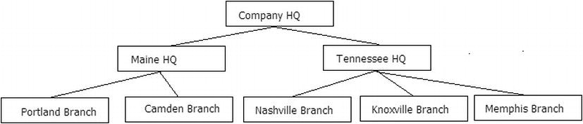
Figure 8-3. Demonstration company hierarchy
The most important thing to understand when dealing with trees in SQL Server is that the most efficient way to work with trees in a procedural language is not the most efficient way to work with data in a set-based relational language. For example, if you were searching a tree in a functional language, you would likely use a recursive algorithm where you traverse the tree one node at a time, from the topmost item, down to the lowest in the tree, and then work your way around to all of the nodes. In Figure 8-4, I show this for the left side of the tree.
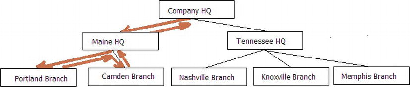
Figure 8-4. Sample tree structure searched depth first
This is referred to as a depth-first search and is really fast when the language is optimized for single-instance-at-a-time access, particularly when you can load the entire tree into RAM. If you attempted to implement this using T-SQL, you would find that it is very slow, as most any iterative processing can be. In SQL, we use what is called a breadth-first search that can be scaled to many more nodes, because the number of queries is limited to the number of levels in the hierarchy. The limitations here pertain to the size of the temporary storage needed and how many rows you end up with on each level. Joining to an unindexed temporary set is bad in your code, and it is not good in SQL Server’s algorithms either.
A tree can be broken down into levels, from the parent row that you are interested in. From there, the levels increase as you are one level away from the parent, as shown in Figure 8-5.
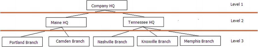
Figure 8-5. Sample tree structure with levels
Now, working with this structure will deal with each level as a separate set, joined to the matching results from the previous level. You iterate one level at a time, matching rows from one level to the next. This reduces the number of queries to use the data down to three, rather than a minimum of eight, plus the overhead of going back and forth from parent to child. To demonstrate working with adjacency list tables, let’s create a table to represent a hierarchy of companies that are parent to one another. The goal of our table will be to implement the structure, as shown in Figure 8-6.
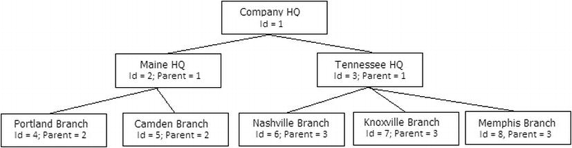
Figure 8-6. Diagram of basic adjacency list
So we will create the following table:
CREATE SCHEMA corporate;
GO
CREATE TABLE corporate.company
(
companyId int NOT NULL CONSTRAINT PKcompany primary key,
name varchar(20) NOT NULL CONSTRAINT AKcompany_name UNIQUE,
parentCompanyId int null
CONSTRAINT company$isParentOf$company REFERENCES corporate.company(companyId)
);
Then, I will load data to set up a table like the graphic in Figure 8-3:
INSERT INTO corporate.company (companyId, name, parentCompanyId)
VALUES (1, 'Company HQ', NULL),
(2, 'Maine HQ',1), (3, 'Tennessee HQ',1),
(4, 'Nashville Branch',3), (5, 'Knoxville Branch',3),
(6, 'Memphis Branch',3), (7, 'Portland Branch',2),
(8, 'Camden Branch',2);
Now, taking a look at the data
SELECT *
FROM corporate.company;
returns:
| companyId | name | parentCompanyId |
| --------- | ---------------- | --------------- |
| 1 | Company HQ | NULL |
| 2 | Maine HQ | 1 |
| 3 | Tennessee HQ | 1 |
| 4 | Nashville Branch | 3 |
| 5 | Knoxville Branch | 3 |
| 6 | Memphis Branch | 3 |
| 7 | Portland Branch | 2 |
| 8 | Camden Branch | 2 |
Now, dealing with this data in a hierarchical manner is pretty simple. In the next code, we will write a query to get the children of a given node and add a column to the output that shows the hierarchy. I have commented the code to show what I was doing, but it is fairly straightforward how this code works:
--getting the children of a row (or ancestors with slight mod to query)
DECLARE @companyId int = <set me>;
;WITH companyHierarchy(companyId, parentCompanyId, treelevel, hierarchy)
AS
(
--gets the top level in hierarchy we want. The hierarchy column
--will show the row's place in the hierarchy from this query only
--not in the overall reality of the row's place in the table
SELECT companyID, parentCompanyId,
1 as treelevel, CAST(companyId as varchar(max)) AS hierarchy
FROM corporate.company
WHERE companyId=@companyId
UNION ALL
--joins back to the CTE to recursively retrieve the rows
--note that treelevel is incremented on each iteration
SELECT company.companyID, company.parentCompanyId,
treelevel + 1 as treelevel,
hierarchy + '' +cast(company.companyId AS varchar(20)) as hierarchy
FROM corporate.company
INNER JOIN companyHierarchy
--use to get children
on company.parentCompanyId= companyHierarchy.companyID
--use to get parents
--on company.CompanyId= companyHierarchy.parentcompanyID
)
--return results from the CTE, joining to the company data to get the
--company name
SELECT company.companyID,company.name,
companyHierarchy.treelevel, companyHierarchy.hierarchy
FROM corporate.company
INNER JOIN companyHierarchy
ON company.companyID = companyHierarchy.companyID
ORDER BY hierarchy;
Running this code with @companyId = 1, you will get the following:
| companyID | name | treelevel | hierarchy |
| --------- | --------------- | --------- | ---------- |
| 1 | Company HQ | 1 | 1 |
| 2 | Maine HQ | 2 | 12 |
| 7 | Portland Branch | 3 | 127 |
| 8 | Camden Branch | 3 | 128 |
| 3 | Tennessee HQ | 2 | 13 |
| 4 | Nashville Branch | 3 | 134 |
| 5 | Knoxville Branch | 3 | 135 |
| 6 | Memphis Branch | 3 | 136 |
![]() Tip Make a note of the hierarchy output here. This is very similar the data used by the path method and will show up in the hierarchyId examples as well.
Tip Make a note of the hierarchy output here. This is very similar the data used by the path method and will show up in the hierarchyId examples as well.
The hierarchy column shows you the position of each of the children of the 'Company HQ' row, and since this is the only row with a null parentCompanyId, you don’t have to start at the top; you can start in the middle. For example, the 'Tennessee HQ'(@companyId = 3) row would return
| companyID | name | treelevel | hierarchy |
| --------- | ---------------- | --------- | ----------- |
| 3 | Tennessee HQ | 1 | 3 |
| 4 | Nashville Branch | 2 | 34 |
| 5 | Knoxville Branch | 2 | 35 |
| 6 | Memphis Branch | 2 | 36 |
If you want to get the parents of a row, you need to make just a small change to the code. Instead of looking for rows in the CTE that match the companyId of the parentCompanyId, you look for rows where the parentCompanyId in the CTE matches the companyId. I left in some code with comments:
--use to get children
ON company.parentCompanyId= companyHierarchy.companyID
--use to get parents
--ON company.CompanyId= companyHierarchy.parentcompanyID
Comment out the first ON, and uncomment the second one:
--use to get children
--ON company.parentCompanyId= companyHierarchy.companyID
--use to get parents
ON company.CompanyId= companyHierarchy.parentcompanyID
And set @companyId to a row with parents, such as 4. Running this you will get
| companyID | name | treelevel | hierarchy |
| --------- | ---------------- | --------- | --------- |
| 4 | Nashville Branch | 1 | 4 |
| 3 | Tennessee HQ | 2 | 43 |
| 1 | Company HQ | 3 | 431 |
The hierarchy column now shows the relationship of the row to the starting point in the query, not it’s place in the tree. Hence, it seems backward, but thinking back to the breadth first searching approach, you can see that on each level, the hierarchy columns in all examples have added data for each iteration.
I should also make note of one issue with hierarchies, and that is circular references. We could easily have the following situation occur:
ObjectId ParentId
-------- --------
1 3
2 1
3 2
In this case, anyone writing a recursive type query would get into an infinite loop because every row has a parent, and the cycle never ends. This is particularly dangerous if you limit recursion on a CTE (via the MAXRECURSION hint) and you stop after N iterations rather than failing, and hence never noticing.
Graphs (Multiparent Hierarchies)
Querying graphs (and in fact, hierarchies as well) are a very complex topic that is well beyond the scope of this book and chapter. It is my goal at this point to demonstrate how to model and implement graphs and leave the job of querying them to an advanced query book.
The most common example of a graph is a product breakdown. Say you have part A, and you have two assemblies that use this part. So the two assemblies are parents of part A. Using an adjacency list embedded in the table with the data you cannot represent anything other than a tree. We split the data from the implementation of the hierarchy. As an example, consider the following schema with parts and assemblies.
First, we create a table for the parts:
CREATE SCHEMA Parts;
GO
CREATE TABLE Parts.Part
(
PartId int NOT NULL CONSTRAINT PKPartsPart PRIMARY KEY,
PartNumber char(5) NOT NULL CONSTRAINT AKPartsPart UNIQUE,
Name varchar(20) NULL
);
Then, we load in some simple data:
INSERT INTO Parts.Part (PartId, PartNumber,Name)
VALUES (1,'00001','Screw'),(2,'00002','Piece of Wood'),
(3,'00003','Tape'),(4,'00004','Screw and Tape'),
(5,'00005','Wood with Tape'),
Next, a table to hold the part containership setup:
CREATE TABLE Parts.Assembly
(
PartId int NOT NULL
CONSTRAINT FKPartsAssembly$contains$PartsPart
REFERENCES Parts.Part(PartId),
ContainsPartId int NOT NULL
CONSTRAINT FKPartsAssembly$isContainedBy$PartsPart
REFERENCES Parts.Part(PartId),
CONSTRAINT PKPartsAssembly PRIMARY KEY (PartId, ContainsPartId),
);
Now, you can load in the data for the Screw and Tape part, by making the part with partId 4 a parent to 1 and 3:
INSERT INTO PARTS.Assembly(PartId,ContainsPartId)
VALUES (4,1),(4,3);
Next, you can do the same thing for the Wood with Tape part:
INSERT INTO Parts.Assembly(PartId,ContainsPartId)
VALUES (5,1),(4,2);
Using a graph can be simplified by dealing with each individual tree independently of one another by simply picking a parent and delving down. Cycles should be avoided, but it should be noted that the same part could end up being used at different levels in the hierarchy. The biggest issue is making sure that you don’t double count data because of the parent to child cardinality that is greater than 1. Graph coding is a very complex topic that I won’t go into here in any depth, while modeling them is relatively straightforward.
Implementing the Hierarchy Using the hierarchyTypeId Type
In SQL Server 2008, Microsoft added a new datatype called hierarchyTypeId. It is used to do some of the heavy lifting of dealing with hierarchies. It has some definite benefits in that it makes queries on hierarchies fairly easier, but it has some difficulties as well.
The primary downside to the hierarchyId datatype is that it is not as simple to work with for some of the basic tasks as is the self-referencing column. Putting data in this table will not be as easy as it was for that method (recall all of the data was inserted in a single statement, this will not be possible for the hierarchyId solution). However, on the bright side, the types of things that are harder with using a self-referencing column will be notably easier, but some of the hierarchyId operations are not what you would consider natural at all.
As an example, I will set up an alternate company table named corporate2 where I will implement the same table as in the previous example using hierarchyId instead of the adjacency list.a hierarchy of companies:
CREATE TABLE corporate.company2
(
companyOrgNode hierarchyId not null
CONSTRAINT AKcompany UNIQUE,
companyId int NOT NULL CONSTRAINT PKcompany2 primary key,
name varchar(20) NOT NULL CONSTRAINT AKcompany2_name UNIQUE,
);
To insert a root node (with no parent), you use the GetRoot() method of the hierarchyId type without assigning it to a variable:
INSERT corporate.company2 (companyOrgNode, CompanyId, Name)
VALUES (hierarchyid::GetRoot(), 1, 'Company HQ'),
To insert child nodes, you need to get a reference to the parentCompanyOrgNode that you want to add, then find its child with the largest companyOrgNode value, and finally, use the getDecendant() method of the companyOrgNode to have it generate the new value. I have encapsulated it into the following procedure (based on the procedure in the tutorials from books online, with some additions to support root nodes and single threaded inserts, to avoid deadlocks and/or unique key violations), and comments to explain how the code works:
CREATE PROCEDURE corporate.company2$insert(@companyId int, @parentCompanyId int,
@name varchar(20))
AS
BEGIN
SET NOCOUNT ON
--the last child will be used when generating the next node,
--and the parent is used to set the parent in the insert
DECLARE @lastChildofParentOrgNode hierarchyid,
@parentCompanyOrgNode hierarchyid;
IF @parentCompanyId IS not null
BEGIN
SET @parentCompanyOrgNode =
( SELECT companyOrgNode
FROM corporate.company2
WHERE companyID = @parentCompanyId)
IF @parentCompanyOrgNode is null
BEGIN
THROW 50000, 'Invalid parentCompanyId passed in',16;
RETURN -100;
END
END
BEGIN TRANSACTION;
--get the last child of the parent you passed in if one exists
SELECT @lastChildofParentOrgNode = max(companyOrgNode)
FROM corporate.company2 (UPDLOCK) --compatibile with shared, but blocks
--other connections trying to get an UPDLOCK
WHERE companyOrgNode.GetAncestor(1) =@parentCompanyOrgNode ;
--getDecendant will give you the next node that is greater than
--the one passed in. Since the value was the max in the table, the
--getDescendant Method returns the next one
INSERT corporate.company2 (companyOrgNode, companyId, name)
--the coalesce puts the row as a NULL this will be a root node
--invalid parentCompanyId values were tossed out earlier
SELECT COALESCE(@parentCompanyOrgNode.GetDescendant(
@lastChildofParentOrgNode, NULL),hierarchyid::GetRoot())
,@companyId, @name;
COMMIT;
END
Now, create the rest of the rows:
--exec corporate.company2$insert @companyId = 1, @parentCompanyId = NULL,
-- @name = 'Company HQ'; --already created
exec corporate.company2$insert @companyId = 2, @parentCompanyId = 1,
@name = 'Maine HQ';
exec corporate.company2$insert @companyId = 3, @parentCompanyId = 1,
@name = 'Tennessee HQ';
exec corporate.company2$insert @companyId = 4, @parentCompanyId = 3,
@name = 'Knoxville Branch';
exec corporate.company2$insert @companyId = 5, @parentCompanyId = 3,
@name = 'Memphis Branch';
exec corporate.company2$insert @companyId = 6, @parentCompanyId = 2,
@name = 'Portland Branch';
exec corporate.company2$insert @companyId = 7, @parentCompanyId = 2,
@name = 'Camden Branch';
You can see the data in its raw format here:
SELECT companyOrgNode, companyId, name
FROM corporate.company2;
This returns a fairly uninteresting result set, particularly since the companyOrgNode value is useless in this untranslated format:
| companyOrgNode | companyId | name |
| -------------- | --------- | ---------------- |
| 0x | 1 | Company HQ |
| 0x58 | 2 | Maine HQ |
| 0x68 | 3 | Tennessee HQ |
| 0x6AC0 | 4 | Knoxville Branch |
| 0x6B40 | 5 | Nashville Branch |
| 0x6BC0 | 6 | Memphis Branch |
| 0x5AC0 | 7 | Portland Branch |
| 0x5B40 | 8 | Camden Branch |
But this is not the most interesting way to view the data. The type includes methods to get the level, the hierarchy, and more:
SELECT companyId, companyOrgNode.GetLevel() as level,
name, companyOrgNode.ToString() as hierarchy
FROM corporate.company2;
which can be really useful in queries:
| companyId | level | name | hierarchy |
| --------- | ----- | ---------------- | --------- |
| 1 | 0 | Company HQ | / |
| 2 | 1 | Maine HQ | /1/ |
| 3 | 1 | Tennessee HQ | /2/ |
| 4 | 2 | Knoxville Branch | /2/1/ |
| 5 | 2 | Memphis Branch | /2/2/ |
| 6 | 2 | Portland Branch | /1/1/ |
| 7 | 2 | Camden Branch | /1/2/ |
Getting all of the children of a node is far easier than it was with the previous method. The hierarchyId type has an IsDecendantOf method you can use. For example, to get the children of companyId = 3, use the following:
DECLARE @companyId int = 3;
SELECT Target.companyId, Target.name, Target.companyOrgNode.ToString() as hierarchy
FROM corporate.company2 AS Target
JOIN corporate.company2 AS SearchFor
ON SearchFor.companyId = @companyId
AND Target.companyOrgNode.IsDescendantOf
(SearchFor.companyOrgNode) = 1;
This returns
companyId name hierarchy
---------- ------------- -----------
3 Tennessee HQ/2/
4 Knoxville Branch /2/1/
5 Memphis Branch /2/2/
What is nice is that you can see in the hierarchy the row’s position in the overall hierarchy without losing how it fits into the current results. In the opposite direction, getting the parents of a row isn’t much more difficult. You basically just switch the position of the SearchFor and the Target in the ON clause:
DECLARE @companyId int = 3;
SELECT Target.companyId, Target.name, Target.companyOrgNode.ToString() as hierarchy
FROM corporate.company2 AS Target
JOIN corporate.company2 AS SearchFor
ON SearchFor.companyId = @companyId
AND SearchFor.companyOrgNode.IsDescendantOf
(Target.companyOrgNode) = 1;
This returns
companyId name hierarchy
--------- ------------ ---------
1 Company HQ /
3 Tennessee HQ /2/
This query is a bit easier to understand than the recursive CTEs we previously needed to work with. And this is not all that the datatype gives you. This chapter and section are meant to introduce topics, not be a complete reference. Check out Books Online for a full reference to hierarchyId.
However, while some of the usage is easier, using hierarchyId some negatives, most particularly when moving a node from one parent to another. There is a reparent method for hierarchyId, but it only works on one node at a time. To reparent a row (if, say, Oliver is now reporting to Cindy rather than Bobby), you will have to reparent all of the people that work for Oliver as well. In the adjacency model, simply moving modifying one row can move all rows at once.
Alternative Methods/Query Optimizations
Dealing with hierarchies in relational data has long been a well trod topic. As such, a lot has been written on the subject of hierarchies and quite a few other techniques that have been implemented. In this section, I will give an overview of three other ways of dealing with hierarchies that have been and will continue to be used in designs:
- Path technique : In this method, which is similar to using hierarchyId, you store the path from the child to the parent in a formatted text string.
- Nested sets: Use the position in the tree to allow you to get children or parents of a row very quickly.
- Kimball helper table : Basically, this stores a row for every single path from parent to child. It’s great for reads but tough to maintain and was developed for read-only situations, like read-only databases.
Each of these methods has benefits. Each is more difficult to maintain than a simple adjacency model or even the hierarchyId solution but can offer benefits in different situations. In the following sections, I am going to give a brief illustrative overview of each. In the downloads for the book, each of these will have example code that is not presented in the book in a separate file from the primary chapter example file.
Path Technique
The path technique is pretty much the manual version of the hierarchy method. In it, you store the path from the child to the parent. Using our hierarchy that we have used so, to implement the path method, we could use the set of data in Figure 8-7. Note that each of the tags in the hierarchy will use the surrogate key for the key values in the path. In Figure 8-7, I have included a diagram of the hierarchy implemented with the path value set for our design.
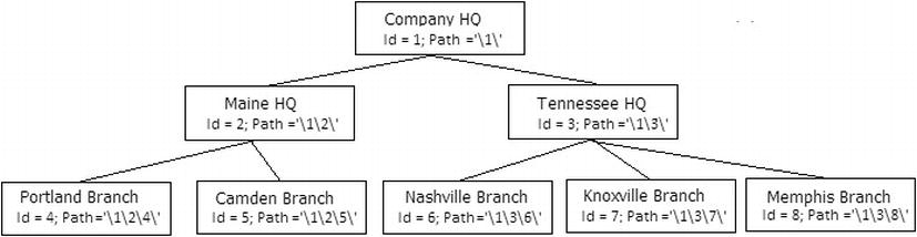
Figure 8-7. Sample hierarchy diagram with values for the path technique
With the path in this manner, you can find all of the children of a row using the path in a like expression. For example, to get the children of the Main HQ node, you can use a WHERE clause such as WHERE Path LIKE '12\%' to get the children, and the path to the parents is directly in the path too. So the parents of the Portland Branch, whose path is '124' are '12' and '1'.
The path method has a bit of an issue with indexing, since you are constantly doing substrings. But they are usually substrings starting with the beginning of the string, so it can be fairly performant. Of course, you have to maintain the hierarchy manually, so it can be fairly annoying to use and maintain this method like this. Generally, hierarchyId seems to be a better fit since it does a good bit of the work for you rather than managing it yourself manually.
One of the more clever methods was created in 1992 by Michael J. Kamfonas. It was introduced in an article named “Recursive Hierarchies: The Relational Taboo!” in The Relational Journal, October/November 1992. You can still find it on his web site, www.kamfonas.com . It is also a favorite of Joe Celko who has written a book about hierarchies named Joe Celko’s Trees and Hierarchies in SQL for Smarties (Morgan Kaufmann, 2004); check it out for further reading about this and other types of hierarchies.
The basics of the method is that you organize the tree by including pointers to the left and right of the current node, enabling you to do math to determine the position of an item in the tree. Again, going back to our company hierarchy, the structure would be as shown in Figure 8-8:

Figure 8-8. Sample hierarchy diagram with values for the nested sests technique
This has the value of now being able to determine children and parents of a node very quickly. To find the children of Maine HQ, you would say WHERE Left > 2 and Right < 7. No matter how deep the hierarchy, there is no traversing the hierarchy at all, just simple math. To find the parents of Maine HQ, you simple need to look for the case WHERE Left < 2 and Right > 7.
Adding a node has a slight negative effect of needing to update all rows to the right of the node, increasing their Right value, since every single row is a part of the structure. Deleting a node will require decrementing the Right value. Even reparenting becomes a math problem, just requiring you to update the linking pointers. Probably the biggest downside is that it is not a very natural way to work with the data, since you don’t have a link directly from parent to child to navigate.
Finally, in a method that is going to be the most complex to manage (but in most cases, the fastest to query), you can use a method that Ralph Kimball created for dealing with hierarchies, particularly in a data warehousing/read-intensive setting, but it could be useful in an OLTP setting if the hierarchy is stable. Going back to our adjacency list implementation, shown in Figure 8-9, assume we already have this implemented in SQL.

Figure 8-9. Sample hierarchy diagram with values for the adjacency list technique repeated for the Kimball helper table method
To implement this method, you will use a table of data that describes the hierarchy with one row per parent to child relationship, for every level of the hierarchy. So there would be a row for Company HQ to Maine HQ, Company HQ to Portland Branch, etc. The helper table provides the details about distance from parent, if it is a root node or a leaf node. So, for the leftmost four items (1, 2, 4, 5) in the tree, we would get the following table.
| ParentId | ChildId | Distance | ParentRootNodeFlag | ChildLeafNodeFlag |
| -------- | -------- | -------- | ------------------ | ----------------- |
| 1 | 2 | 1 | 1 | 0 |
| 1 | 4 | 2 | 1 | 1 |
| 1 | 5 | 2 | 1 | 1 |
| 2 | 4 | 1 | 0 | 1 |
| 2 | 5 | 1 | 0 | 1 |
The power of this technique is that now you can simply ask for all children of 1 by looking for WHERE ParentId = 1, or you can look for direct descendents of 2 by saying WHERE ParentId = 2 and Distance = 1. And you can look for all leaf notes of the parent by querying WHERE ParentId = 1 and ChildLeafNode = 1.
The obvious downfall of this method is simple. It is hideous to maintain if the structure is frequently modified. To be honest, Kimball’s purpose for the method was to optimize relational usage of hierarchies in the data warehouse, which is maintained by ETL. For this sort of purpose, this method should be the quickest, because all queries will be almost completely based on simple relational queries. Of all of the methods, this one will be the most natural for users, while being the less desirable to the team that has to maintain the data.
Images, Documents, and Other Files, Oh My
Storing large binary objects, such PDFs, images, and really any kind of object you might find in your Windows file system is generally not the historic domain of the relational database. As time has passed, however, it is becoming more and more commonplace.
When discussing how to store large objects in SQL Server, generally speaking this would be in reference to data that is (obviously) large but usually in some form of binary format that is not naturally modified using common T-SQL statements, for example, a picture or a formatted document. Most of the time, this is not considering simple text data or even formatted, semistructured text, or even highly structured text such as XML. SQL Server has an XML type for storing XML data (including the ability to index fields in the XML document), and it also has varchar(max)/nvarchar(max) types for storing very large “plain” text data. Of course, sometimes, you will want to store text data in the form of a Windows text file to allow users to manage the data naturally. When deciding a way to store binary data in SQL Server, there are typically two ways that are available:
Prior to 2008, the question was pretty easy to answer indeed. Almost always, the most reasonable solution was to store files in the file system and just store a reference to the data in a varchar column. In SQL Server 2008, Microsoft implemented a new type of binary storage called a filestream , which allows binary data to be stored in the file system as actual files, which makes accessing this data from a client much faster than if it were stored in a binary column in SQL Server. In SQL Server 2011, the picture improves even more to give you a method to store any file data in the server that gives you access to the data using what looks like a typical network share. In all cases, you can deal with the data in T-SQL as before, and even that may be improved, though you cannot do partial writes to the values like you can in a basic varbinary(max) column.
In the 2005 edition of this book, I separated the choice between the two possible ways to store binaries into one main simple reason to choose one or the other: transactional integrity. If you required transaction integrity, you use SQL Server’s storage engine, regardless of the cost you would incur. If transaction integrity isn’t tremendously important, use the file system. For example, if you were just storing an image that a user could go out and edit, leaving it with the same name, the file system is perfectly natural. Performance was a consideration, but if you needed performance, you could write the data to the storage engine first and then regularly refresh the image to the file system and use it from a cache.
In SQL Server 2008, the choice was expanded to include not only basic varbinary(max) columns but now included what is known as a filestream columns. Filestream column data is saved in the filesystem as files, which can be very fast because you can access the data using a special windows share, but the accessor must be within a transaction at the time. It can be useful in some situations, but it requires external APIs to make it work in a natural manner. The setup is pretty easy; first, you will enable filestream access for the server. For details on this process, check the Books Online topic “Enable and Configure FILESTREAM.” The basics are to enable go to SQL Server Configuration Manager and choose the SQL Server Instance in SQL Server Services. Open the properties, and choose the FILESTREAM tab, as shown in Figure 8-10.
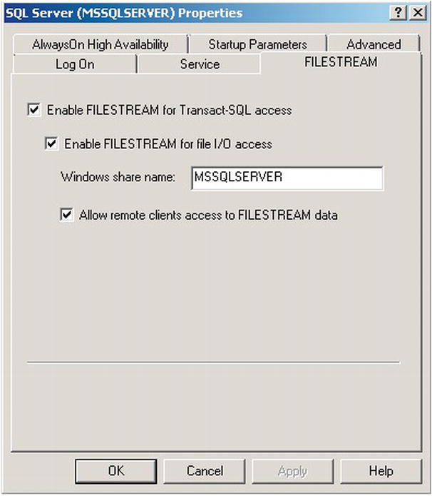
Figure 8-10. Configuring the server for filestream access
The Windows share name will be used to access filetable data later in this chapter. Later in this section, there will be additional configurations based on how the filestream data will be accessed. Next, we create a sample database (instead of using pretty much any database as we have for the rest of this chapter).
CREATE DATABASE FileStorageDemo; --uses basic defaults from model databases
GO
USE FileStorageDemo;
GO
--will cover filegroups more in the chapter 10 on structures
ALTER DATABASE FileStorageDemo ADD
FILEGROUP FilestreamData CONTAINS FILESTREAM;
![]() Tip You cannot use filestream data in a database that also needs to use snapshot isolation level or that implements the READ_COMMITTED_SNAPSHOT database option.
Tip You cannot use filestream data in a database that also needs to use snapshot isolation level or that implements the READ_COMMITTED_SNAPSHOT database option.
Next, add a “file” to the database that is actually a directory for the filestream files:
ALTER DATABASE FileStorageDemo ADD FILE (
NAME = FilestreamDataFile1,
FILENAME = 'c:sqlfilestream') --directory cannot yet exist
TO FILEGROUP FilestreamData;
Now, you can create a table and include a varbinary(max) column with the keyword FILESTREAM after the datatype declaration. Note, too, that we need a unique identifier column with the ROWGUIDCOL property that is used by some of the system processes as a kind of special surrogate key.
CREATE TABLE TestSimpleFileStream
(
TestSimpleFilestreamId INT NOT NULL
CONSTRAINT PKTestSimpleFileStream PRIMARY KEY,
FileStreamColumn VARBINARY(MAX) FILESTREAM NULL,
RowGuid uniqueidentifier NOT NULL ROWGUIDCOL DEFAULT (NewId()) UNIQUE
FILESTREAM_ON FilestreamData; --optional, goes to default otherwise
);
It is as simple as that. You can use the data exactly like it is in SQL Server, as you can create the data using as simple query:
INSERT INTO TestSimpleFileStream(TestSimpleFilestreamId,FileStreamColumn)
SELECT 1, CAST('This is an exciting example' as varbinary(max));
and see it using a typical SELECT:
SELECT TestSimpleFilestreamId,FileStreamColumn,
CAST(FileStreamColumn as varchar(40)) as FileStreamText
FROM TestSimpleFilestream;
I won’t go any deeper into filestreams, because all of the more interesting bits of the technology from here are external to SQL Server in API code, which is well beyond the purpose of this section, which is to show you the basics of setting up the filestream column in your structures.
In SQL Server 2012, we get a new feature for storing binary files called a filetable. A filetable is a special type of table that you can access using T-SQL or directly from the file system using the share we set up earlier in this section named MSSQLSERVER . One of the nice things for us is that we will actually be able to see the file that we create in a very natural manner.
The first thing you need to do is enable filetable access via Windows if it hasn’t been done before (it won’t error or anything if it has already been run):
EXEC sp_configure filestream_access_level, 2;
RECONFIGURE;
The domain for the parameter that is valued 2 (from Books Online) is 0: Disable filestream for the instance; 1: enable filestream for T-SQL; 2: Enable T-SQL and Win32 streaming access. Then, you enable and set up filetable style filestream in the database:
ALTER database FileStorageDemo
SET FILESTREAM (NON_TRANSACTED_ACCESS = FULL,
DIRECTORY_NAME = N'ProSQLServer2012DBDesign'),
The setting NON_TRANSACTED_ACCESS lets you set if users can change data when accessing the data as a Windows share. The changes are not transactionally safe, so data stored in a filetable is not as safe as using a simple varbinary(max) or even one using the filestream attribute. It behaves pretty much like data on any file server, except that it will be backed up with the database, and you can easily associate a file with other data in the server using common relational constructs. The DIRECTORY_NAME parameter is there to add to the path you will access the data (this will be demonstrated later in this section).
The syntax for creating the filetable is pretty simple:
CREATE TABLE dbo.FileTableTest AS FILETABLE
WITH (
FILETABLE_DIRECTORY = 'FileTableTest',
FILETABLE_COLLATE_FILENAME = database_default
);
The FILETABLE_DIRECTORY is the final part of the path for access, and the FILETABLE_COLLATE_FILENAME determines the collation that the filenames will be treated as. It must be case insensitive, because Windows directories are case insensitive. I won’t go in depth with all of the columns and settings, but suffice it to say that the filetable is based on a fixed table schema, and you can access it much like a common table. There are two types of rows, directories, and files. Creating a directory is easy. For example, if you wanted to create directory for Project 1:
INSERT INTO FiletableTest(name, is_directory)
VALUES ( 'Project 1', 1);
Then, you can view this data in the table:
SELECT stream_id, file_stream, name
FROM FileTableTest
WHERE name = 'Project 1';
This will return (though with a different stream_id):
| stream_id | file_stream | name |
| ------------------------------------ | ---------- | --------- |
| 9BCB8987-1DB4-E011-87C8-000C29992276 | NULL | Project 1 |
stream_id is automatically a unique key that you can relate to with your other tables, allowing you to simply present the user with a “bucket” for storing data. Note that the primary key of the table is the path_locator hierarchyId, but this is a changeable value. The stream_id value shouldn’t ever change, though the file or directory could be moved. Before we go check it out in Windows, let’s add a file to the directory. We will create a simple text file, with a small amount of text:
INSERT INTO FiletableTest(name, is_directory, file_stream)
VALUES ( 'Test.Txt', 0, cast('This is some text' as varbinary(max)));
Then, we can move the file to the directory we just created using the path_locator hierarchyId functionality:
UPDATE FiletableTest
SET path_locator = path_locator.GetReparentedValue( path_locator.GetAncestor(1),
(SELECT path_locator FROM FiletableTest
WHERE name = 'Project 1'
AND parent_path_locator is NULL
AND is_directory = 1))
WHERE name = 'Test.Txt';
Now, go to the share that you have set up and view the directory in Windows. Using the function FileTableRootPath() , you can get the filetable path for the database, in our case, \DENALI-PCMSSQLSERVERProSQLServer2012DBDesign, which is my computer’s name, the MSSQLSERVER we set up in Configuration Manager, and ProSQLServer2012DBDesign from the ALTER DATABASE statement turning on filestream.
Now, concatenating the root to the path for the directory, which can be retrieved from the file_stream column (yes, the value you see when querying it is NULL, which is a bit confusing). Now, execute this:
SELECT CONCAT(FileTableRootPath(),
file_stream.GetFileNamespacePath()) AS FilePath;
FROM dbo.FileTableTest
WHERE name = 'Project 1'
AND parent_path_locator is NULL
AND is_directory = 1;
This returns the following:
FilePath
------------------------------------------------------------------------
\DENALI-PCMSSQLSERVERProSQLServer2012DBDesignFileTableTestProject 1
You can then enter this into Explorer to see something like what’s shown in Figure 8-11 (assuming you have everything configured correctly, of course). Note that security for the Windows share is the same as for the filetable through T-SQL, which you administer the same as with any regular table:
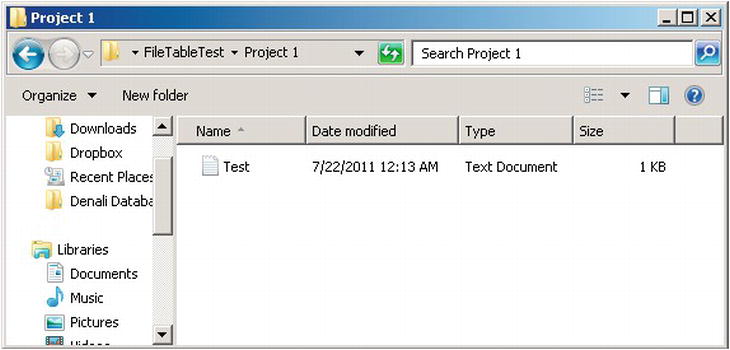
Figure 8-11. Filetable directory opened in Windows Explorer
From here, I would suggest you drop a few files in the directory and check out the metadata for your files in your newly created filetable. It has a lot of possibilities. I will touch more on security in Chapter 9, but the basics are that security is based on Windows Authentication as you have it set up in SQL Server on the table, just like any other table.
![]() Note If you try to use Notepad to access the text file on the same server as the share is located, you will receive an error due to the way notepad accesses files locally. Accessing the file from a remote location using Notepad will work fine.
Note If you try to use Notepad to access the text file on the same server as the share is located, you will receive an error due to the way notepad accesses files locally. Accessing the file from a remote location using Notepad will work fine.
I won’t spend any more time covering the particulars of implementing with filetables. Essentially, with very little trouble, even a fairly basic programmer could provide a directory per client to allow the user to navigate to the directory and get the customer’s associated files. And the files can be backed up with the normal backup operations.
So, mechanics aside, we have discussed essentially four different methods of storing binary data in SQL tables:
- Store a UNC path in a simple character column
- Store the binary data in a simple varbinary(max) column
- Store the binary data in a varbinary(max) using the filestream type
- Store the binary data using a filetable
![]() Tip There is one other type of method of storing large binary values using what is called the Remote Blob Store API. It allows you to use an external storage device to store and manage the images. It is not a typical case, though it will definitely be of interest to people building high-end solutions needing to store blobs on an external device.
Tip There is one other type of method of storing large binary values using what is called the Remote Blob Store API. It allows you to use an external storage device to store and manage the images. It is not a typical case, though it will definitely be of interest to people building high-end solutions needing to store blobs on an external device.
Each of these has some merit, and I will discuss the pros and cons in the following list. Like with any newer, seemingly easier technology, a filetable does feel like it might take the nod for a lot of upcoming uses, but definitely consider the other possibilities when evaluating your needs in the future.
- Transactional integrity : It’s far easier to guarantee that the image is stored and remains stored if it is managed by the storage engine, either as a filestream or as a binary value, than it is if you store the filename and path and have an external application manage the files. A filetable could be used to maintain transactional integrity, but to do so, you will need to disallow nontransaction modifications, which will then limit how much easier it is to work with.
- Consistent backup of image and data: Knowing that the files and the data are in sync is related to transactional integrity. Storing the data in the database, either as a binary columnar value or as a filestream/filetable, ensures that the binary values are backed up with the other database objects. Of course, this can cause your database size to grow very large, so it can be handy to use partial backups of just the data and not the images at times. Filegroups can be restored individually as well, but be careful not to give up integrity for faster backups if the business doesn’t expect it.
- Size : For sheer speed of manipulation, for the typical object size less than 1MB, Books Online suggests using storage in a varchar(max). If objects are going to be more than 2GB, you must use one of the filestream storage types.
- API : Which API is the client using? If the API does not support using the filestream type, you should definitely give it a pass. A filetable will let you treat the file pretty much like it was on any network share, but note that access/modification through the filesystem is not part of a transaction, so if you need the file modification to occur along with other changes as a transaction, it will not do.
- Utilization : How will the data be used? If it is used very frequently, then you would choose either filestream/filetable or file system storage. This could particularly be true for files that need to be read only. Filetable is a pretty nice way to allow the client to view a file in a very natural manner.
- Location of files : Filestream filegroups are located on the same server as the relational files. You cannot specify a UNC path to store the data. For filestream column use, the data, just like a normal filegroup, must be transactionally safe for utilization. (Again, as the preceding note states, there are devices that implement a remote blob store to get around this limitation.)
- Encryption : Encryption is not supported on the data store in filestream filegroups, even when transparent data encryption (TDE) is enabled.
- Security : If the image’s integrity is important to the business process (such as the picture on a security badge that’s displayed to a security guard when a badge is swiped), it’s worth it to pay the extra price for storing the data in the database, where it’s much harder to make a change. (Modifying an image manually in T-SQL is a tremendous chore indeed.) A filetable also has a disadvantage in that implementing row-level security (discussed in Chapter 9 in more detail) using views would not be possible, whereas when using a filestream-based column, you are basically using the data in a SQL-esque manner until you access the file, though still in the context of a transaction.
For three quick examples, consider a movie rental database. In one table, we have a MovieRentalPackage table that represents a particular packaging of a movie for rental. Because this is just the picture of a movie, it is a perfectly valid choice to store a path to the data. This data will simply be used to present electronic browsing of the store’s stock, so if it turns out to not work one time, that is not a big issue. Have a column for the PictureUrl that is varchar(200), as shown in Figure 8-12.
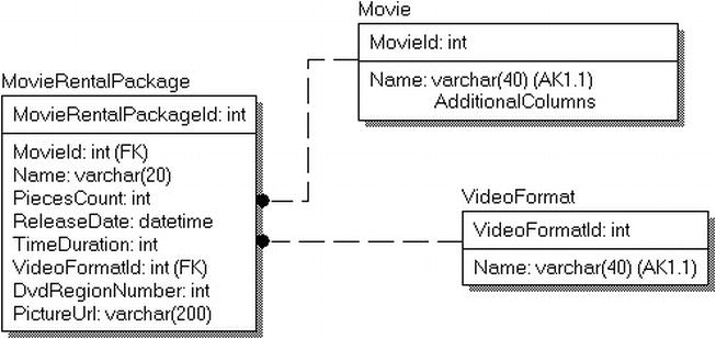
Figure 8-12. MovieRentalPackage table with PictureUrl datatype set as a path to a file
This path might even be on an Internet source where the filename is an HTTP:// address and be located in a web server’s image cache and could be replicated to other web servers. The path may or may not be stored as a full UNC location; it really would depend on your infrastructure needs. The goal will be when the page is fetching data from the server to be able to build a bit of HTML such as this:
SELECT '<img src = "' + MovieRentalPackage.PictureUrl + '">', …
FROM MovieRentalPackage
WHERE MovieId = @MovieId;
If this data were stored in the database as a binary format, it would need to be materialized onto disk as a file first and then used in the page, which is going to be far slower than doing it this way, no matter what your architecture. This is probably not a case where you would want to do this or go through the hoops necessary for filestream access, since transactionally speaking, if the picture link is broken, it would not invalidate the other data, and it is probably not very important. Plus, you will probably want to access this file directly, making the main web screens very fast and easy to code.
An alternative example might be accounts and associated users (see Figure 8-13). To fight fraud, a movie rental chain may decide to start taking customer pictures and comparing them whenever customers rent an item. This data is far more important from a security standpoint and has privacy implications. For this, I’ll use a varbinary(max) for the person’s picture in the database.
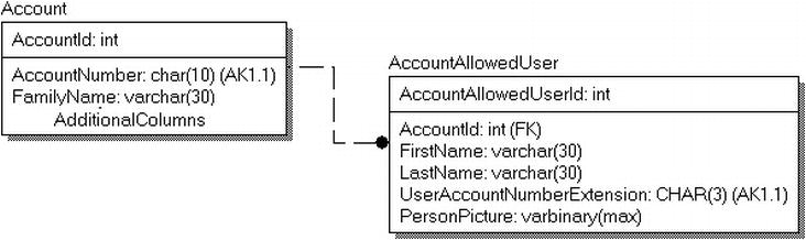
Figure 8-13. Customer table with picture stored as data in the table
At this point, you have definitely decided that transactional integrity is necessary and that you want to retrieve the data directly from the server. The next thing to decide will be whether to employ filestreams. The big questions here would be if your API will support filestreams. If so, it would likely be a very good place to make use of them for sure. Size could play a part in the choice too, though security pictures would likely be less than 1MB anyhow.
Overall, speed probably isn’t a big deal, and even if you needed to take the binary bits and stream them from SQL Server’s normal storage into a file, it would probably still perform well enough since only one image needs to be fetched at a time, and performance will be adequate as long as the image displays before the rental transaction is completed. Don’t get me wrong; the varbinary(max) types aren’t that slow, but performance would be acceptable for these purposes even if they were.
Finally, consider if you wanted to implement a customer file system to store scanned images pertaining to the customer. Not enough significance is given to the data to require it to be managed in a structured manner, but they simply want to be able to create a directory to hold scanned data. The data does need to be kept in sync with the rest of the database. So you could extend your table to include a filetable (AccountFileDirectory in Figure 8-14, with stream_id modeled as primary, even though it is technically a unique constraint in implementation, you can reference an alternate key).
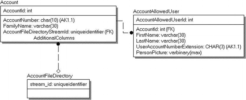
Figure 8-14. Account model extended with an AccountFileDirectory
In this manner, you have included a directory for the account’s files that can be treated like a typical file structure but will be securely located with the account information. This will be not only very usable for the programmer and user alike but also give you the security of knowing the data is backed up with the account files and treated in the same manner as the account information.
One of the interesting changes in database design in SQL Server 2012 is dealing with unstructured file data, and it is a tremendously interesting change. Not everyone needs to store a lot of image data, but if you do, the new filetable feature definitely opens things up for much easier access.
Very often, it is tempting to design more tables than is truly necessary for the system needs, because we get excited and start to design perfection. For example, if you were designing a database to store information about camp activities, it might be tempting to have an individual table for the archery class, the swimming class, and so on, modeling with great detail the activities of each camp activity. If there were 50 activities at the camp, you might have 50 tables, plus a bunch of other tables to tie these 50 together. In the end though, while these tables may not exactly look the same, you will start to notice that every table is used for basically the same thing. Assign an instructor, sign up kids to attend, and add a description. Rather than the system being about each activity, and so needing a model each of the different activities as being different from one another, what you truly needed was to model was the abstraction of a camp activity.
In the end, the goal is to consider where you can combine foundationally similar tables into a single table, particularly when multiple tables are constantly being treated as one, as you would have to do with the 50 camp activity tables, particularly to make sure kids weren’t signing up their friends for every other session just to be funny.
During design, it is useful to look for similarities in utilization, columns, and so on, and consider collapsing multiple tables into one, ending up with a generalization/abstraction of what is truly needed to be modeled. Clearly, however, the biggest problem here is that sometimes you do need to store different information about some of the things your original tables were modeling. For example, if you needed special information about the snorkeling class, you might lose that if you just created one activity abstraction, and heaven knows the goal is not to end up with a table with 200 columns all prefixed with what ought to have been a table in the first place.
In those cases, you can consider using a subclassed entity for certain entities. Take the camp activity model. We include the generalized table for the generic CampActivity , which is where you would associate student and teachers who don’t need special training, and in the subclassed tables, you would include specific information about the snorkeling and archery classes, likely along with the teachers who meet specific criteria, as shown in Figure 8-15.
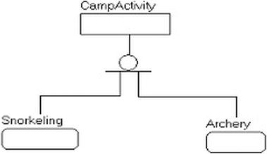
Figure 8-15. Extending generalized entity with specific details as required
As a coded example, we will look at a home inventory system. You have various types of stuff in your house, and you clearly want to inventory everything or at least everything valuable. So would you simply design a table for each type of item? That seems like too much trouble, because most everything you will simply have a description, picture, value, and a receipt. On the other hand, a single table, generalizing all of the items in your house down to a single list seems like it might not be enough for items that you need specific information about, like appraisals and serial numbers.
For example, some jewelry probably ought to be appraised and have the appraisal listed. Electronics and appliances ought to have brand, model, and alternatively, serial numbers captured. So the goal is to generalize a design to the level where you have a basic list of the home inventory that you can list, but you can also print a list of jewelry alone with extra detail or electronics with their information.
So we implement the database as such. First, we create the generic table that holds generic item descriptions:
CREATE SCHEMA Inventory;
GO
CREATE TABLE Inventory.Item
(
ItemId int NOT NULL IDENTITY CONSTRAINT PKInventoryItem PRIMARY KEY,
Name varchar(30) NOT NULL CONSTRAINT AKInventoryItemName UNIQUE,
Type varchar(15) NOT NULL,
Color varchar(15) NOT NULL,
Description varchar(100) NOT NULL,
ApproximateValue numeric(12,2) NULL,
ReceiptImage varbinary(max) NULL,
PhotographicImage varbinary(max) NULL
);
I included two columns for holding an image of the receipt as well as a picture of the item. Like we discussed in the previous section, you might want to use a filetable construct to just allow various electronic items to be associated with this data, but it would probably be sufficient to simply have a picture of the receipt and the item minimally attached to the row for easy use. In the sample data, I always load the data with a simple hex value of 0x001 as a placeholder:
INSERT INTO Inventory.Item
VALUES ('Den Couch','Furniture','Blue','Blue plaid couch, seats 4',450.00,0x001,0x001),
('Den Ottoman','Furniture','Blue','Blue plaid ottoman that goes with couch',
150.00,0x001,0x001),
('40 Inch Sorny TV','Electronics','Black',
'40 Inch Sorny TV, Model R2D12, Serial Number XD49292',
800,0x001,0x001),
('29 Inch JQC TV','Electronics','Black','29 Inch JQC CRTVX29 TV',800,0x001,0x001),
('Mom''s Pearl Necklace','Jewelery','White',
'Appraised for $1300 in June of 2003. 30 inch necklace, was Mom''s',
1300,0x001,0x001);
Checking out the data using the following query:
SELECT Name, Type, Description
FROM Inventory.Item;
We see that we have a good little system, though data isn’t really organized how we need it, because in realistic usage, we will probably need some of the specific data from the descriptions:
| Name | Type | Description |
| -------------------- | ----------- | ----------------------------------- |
| Den Couch | Furniture | Blue plaid couch, seats 4 |
| Den Ottoman | Furniture | Blue plaid ottoman that goes with… |
| 40 Inch Sorny TV | Electronics | 40 Inch Sorny TV, Model R2D12, Ser… |
| 29 Inch JQC TV | Electronics | 29 Inch JQC CRTVX29 TV |
| Mom’s Pearl Necklace | Jewelery | Appraised for $1300 in June of 200… |
At this point, we look at our data and reconsider the design. The two pieces of furniture are fine. We have a picture and a brief description. For the other two items, however, using the data becomes trickier. For electronics, the insurance company is going to want model and serial number for each, but the two TV entries use different formats, and one of them doesn’t capture the serial number. Did they forget to capture it? Or does it not exist?
So, we add subclasses for cases where we need to have more information, to help guide the user as to how to enter data:
CREATE TABLE Inventory.JeweleryItem
(
ItemId int CONSTRAINT PKInventoryJewleryItem PRIMARY KEY
CONSTRAINT FKInventoryJewleryItem$Extends$InventoryItem
REFERENCES Inventory.Item(ItemId),
QualityLevel varchar(10)NOT NULL,
AppraiserName varchar(100) NULL,
AppraisalValue numeric(12,2) NULL,
AppraisalYear char(4) NULL
);
GO
CREATE TABLE Inventory.ElectronicItem
(
ItemId int CONSTRAINT PKInventoryElectronicItem PRIMARY KEY
CONSTRAINT FKInventoryElectronicItem$Extends$InventoryItem
REFERENCES Inventory.Item(ItemId),
BrandName varchar(20) NOT NULL,
ModelNumber varchar(20) NOT NULL,
SerialNumber varchar(20) NULL
);
Now, we adjust the data in the tables to have names that are meaningful to the family, but we can create views of the data that have more or less technical information to provide to other people—first, the two TVs. Note that we still don’t have a serial number, but now, it would be simple to find electronics that have no serial number to tell us that we need to get one:
UPDATE Inventory.Item
SET Description = '40 Inch TV'
WHERE Name = '40 Inch Sorny TV';
GO
INSERT INTO Inventory.ElectronicItem (ItemId, BrandName, ModelNumber, SerialNumber)
SELECT ItemId, 'Sorny','R2D12','XD49393'
FROM Inventory.Item
WHERE Name = '40 Inch Sorny TV';
GO
UPDATE Inventory.Item
SET Description = '29 Inch TV'
WHERE Name = '29 Inch JQC TV';
GO
INSERT INTO Inventory.ElectronicItem(ItemId, BrandName, ModelNumber, SerialNumber)
SELECT ItemId, 'JVC','CRTVX29',NULL
FROM Inventory.Item
WHERE Name = '29 Inch JQC TV';
Finally, we do the same for the jewelry items, adding the appraisal value from the text.
UPDATE Inventory.Item
SET Description = '30 Inch Pearl Neclace'
WHERE Name = 'Mom''s Pearl Necklace';
GO
INSERT INTO Inventory.JeweleryItem (ItemId, QualityLevel, AppraiserName, AppraisalValue,AppraisalYear)
SELECT ItemId, 'Fine','Joey Appraiser',1300,'2003'
FROM Inventory.Item
WHERE Name = 'Mom''s Pearl Necklace';
Looking at the data now, you see the more generic list with names that are more specifically for the person maintaining the list:
SELECT Name, Type, Description
FROM Inventory.Item;
This returns
| Name | Type | Description |
| -------------------- | ----------- | ------------------------------- |
| Den Couch | Furniture | Blue plaid couch, seats 4 |
| Den Ottoman | Furniture | Blue plaid ottoman that goes w… |
| 40 Inch Sorny TV | Electronics | 40 Inch TV |
| 29 Inch JQC TV | Electronics | 29 Inch TV |
| Mom's Pearl Necklace | Jewelery | 30 Inch Pearl Neclace |
And to see specific electronics items with their information, you can use a query such as this, with an inner join to the parent table to get the basic nonspecific information:
SELECTItem.Name, ElectronicItem.BrandName, ElectronicItem.ModelNumber, ElectronicItem.SerialNumber
FROMInventory.ElectronicItem
JOIN Inventory.Item
ON Item.ItemId = ElectronicItem.ItemId;
This returns
| Name | BrandName | ModelNumber | SerialNumber |
| ---------------- | --------- | ----------- | ------------ |
| 40 Inch Sorny TV | Sorny | R2D12 | XD49393 |
| 29 Inch JQC TV | JVC | CRTVX29 | NULL |
Finally, it is also quite common that you may want to see a complete inventory with the specific information, since this is truly the natural way you think of the data and why the typical designer will design the table in a single table no matter what. We return an extended description column this time by formatting the data based on the type of row:
SELECT Name, Description,
CASE Type
WHEN 'Electronics'
THEN 'Brand:' + COALESCE(BrandName,'_______') +
' Model:' + COALESCE(ModelNumber,'________') +
' SerialNumber:' + COALESCE(SerialNumber,'_______')
WHEN 'Jewelery'
THEN 'QualityLevel:' + QualityLevel +
' Appraiser:' + COALESCE(AppraiserName,'_______') +
' AppraisalValue:' +COALESCE(Cast(AppraisalValue as varchar(20)),'_______')
+' AppraisalYear:' + COALESCE(AppraisalYear,'____')
ELSE '' END as ExtendedDescription
FROM Inventory.Item --outer joins because every item will only have one of these if any
LEFT OUTER JOIN Inventory.ElectronicItem
ON Item.ItemId = ElectronicItem.ItemId
LEFT OUTER JOIN Inventory.JeweleryItem
ON Item.ItemId = JeweleryItem.ItemId;
This returns a formatted description:
| Name | Description | ExtendedDescription |
| -------------------- | ------------------------- | -------------------------------------------- |
| Den Couch | Blue plaid couch, seats 4 | |
| Den Ottoman | Blue plaid ottoman that … | |
| 40 Inch Sorny TV | 40 Inch TV | Brand:Sorny Model:R2D12 SerialNumber:XD49393 |
| 29 Inch JQC TV | 29 Inch TV | Brand:JVC Model:CRTVX29 SerialNumber:_______ |
| Mom's Pearl Necklace | 30 Inch Pearl Neclace | NULL |
The point of this section on generalization really goes back to the basic precepts that you design for the user’s needs. If we had created a table per type of item in the house: Inventory.Lamp, Inventory.ClothesHanger, and so on, the process of normalization gets the blame. But the truth is, if you really listen to the user’s needs and model them correctly, you may never need to consider generalizing your objects. However, it is still a good thing to consider, looking for commonality among the objects in your database looking for cases where you could get away with less tables rather than more.
![]() Tip It may seem unnecessary, even for a simple home inventory system to take these extra steps in your design. However, the point I am trying to make here is that if you have rules about how data should look, almost certainly having a column for that data is going to make more sense. Even if your business rule enforcement is as minimal as just using the final query, it will be far more obvious to the end user that the SerialNumber: ___________ value is a missing value that probably needs to be filled in.
Tip It may seem unnecessary, even for a simple home inventory system to take these extra steps in your design. However, the point I am trying to make here is that if you have rules about how data should look, almost certainly having a column for that data is going to make more sense. Even if your business rule enforcement is as minimal as just using the final query, it will be far more obvious to the end user that the SerialNumber: ___________ value is a missing value that probably needs to be filled in.
One of the common problems that has no comfortable solution is giving users a method to expand the catalog of values they can store without losing control of the database design. The biggest issue is the integrity of the data that they want to store in this database, in that it is very rare that you want to store data and not use it to make decisions. In this section, I will explore a couple of the common methods for doing expanding the data catalog by the end user.
As I have tried to make clear throughout the rest of the book so far, relational tables are not meant to be flexible. SQL Server code is not really meant to be overly flexible. T-SQL as a language is not made for flexibility (at least not from the standpoint of producing reliable databases that produce expected results and producing good performance while protecting the quality of the data, which I have said many times is almost always the most important thing).
Unfortunately, reality is that users want flexibility, and frankly, you can’t tell users that they can’t get what they want, when they want it, and in the form they want it. As an architect, I want to give the users what they want, within the confines of reality and sensibility, so it is necessary to ascertain some method of giving the user the flexibility they demand, along with methods to deal with this data in a manner that feels good to them. The technique used to solve this problem is pretty simple. It requires the design to be flexible enough to morph to the needs of the user, without the intervention of a database programmer manually changing the catalog. But with all problems, there are generally a couple of solutions that can be used to improve them.
![]() Note I will specifically speak only of methods that are methods that allow you to work with the relational engine in a seminatural manner. There are others, such using an XML column that can be used, but they require you to use completely different methods for dealing with the data.
Note I will specifically speak only of methods that are methods that allow you to work with the relational engine in a seminatural manner. There are others, such using an XML column that can be used, but they require you to use completely different methods for dealing with the data.
The methods I will demonstrate are as follows:
- Big old list of generic columns
- Entity-attribute-value (EAV)
- Adding columns to the table, likely using sparse columns
The last time I had this type of need was to gather the properties on networking equipment. Each router, modem, and so on for a network has various properties (and hundreds or thousands of them at that). For this section, I will present this example as three different examples.
The basis of this example will be a simple table called Equipment . It will have a surrogate key and a tag that will identify it. It is created using the following code:
CREATE SCHEMA Hardware;
GO
CREATE TABLE Hardware.Equipment
(
EquipmentId int NOT NULL
CONSTRAINT PKHardwareEquipment PRIMARY KEY,
EquipmentTag varchar(10) NOT NULL
CONSTRAINT AKHardwareEquipment UNIQUE,
EquipmentType varchar(10)
);
GO
INSERT INTO Hardware.Equipment
VALUES (1,'CLAWHAMMER','Hammer'),
(2,'HANDSAW','Saw'),
(3,'POWERDRILL','PowerTool'),
By this point in this book, you should know that this is not how the whole table would look in the actual solutions, but these three columns will give you enough to build an example from.
Big Old List of Generic Columns
The basics of this plan is to create your normalized tables, make sure you have everything nicely normalized, and then, just in case the user wants to store “additional” information, create a bunch of generic columns. This sort of tactic is quite common in product-offering databases, where the people who are building the database are trying to make sure that the end users have some space in the tool for their custom application.
For our example, adjusting the Equipment table, someone might implement a set of columns in their table such as the following alternate version of our original table, shown in Figure 8-16.
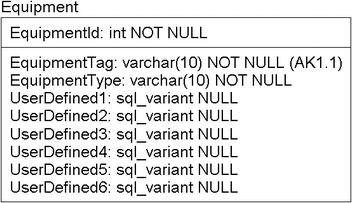
Figure 8-16. Equipment table with UserDefined columns
On the good hand, the end user has a place to store some values that they might need. On the not so good hand, without some very stringent corporate policy, these columns will just be used in any manner that each user decides. This is often the case, which leads to chaos when using this data in SQL. In the best case, userDefined1 is where users always put the schmeglin number, and the second the cooflin diameter or some other value. If the programmer building the user interface is “clever,” he could give names to these columns in some metadata that he defines so that they show up on the screen with usable names.
The next problem, though, comes for the person who is trying to query the data, because knowing what each column means is too often a mystery. If you are lucky, there will be metadata you can query and then build views, and so on. The problem is that you have put the impetus on the end user to know this before using the data, whereas in the other methods, the definition will be part of even creating storage points, and the usage of them will be slightly more natural, if sometimes a bit more troublesome.
From a physical implementation/tuning point of view, the problem with this is that by adding these sql_variant columns, you are potentially bloating your base table, making any scans of the table take longer, increasing page splits, and so on. I won’t produce sample code for this because it would be my goal to dissuade you from using this pattern of implementing user-defined data, but it is a technique that is commonly done.
The next method of implementing user-specified data is using the entity-attribute-value (EAV) method. These are also known by a few different names, such as property tables, loose schemas, or open schema. In 2005 and earlier, this technique was generally considered the default method of implementing a table to allow users to configure their own storage and is still a commonly used pattern.
The basic idea behind this method is to have another related table associated with the table you want to add information about. This table will hold the values that you want to store. Then, you can either include the name of the attribute in the property table or (as I will do) have a table that defines the basic properties of a property.
Considering our needs with equipment, I will use the model shown in Figure 8-17.
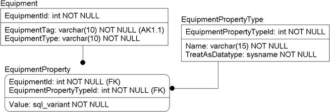
Figure 8-17. Property schema for storing equipment properties with unknown attributes
Using these values in queries isn’t a natural task at all, and as such, you should avoid loose schemas like this unless absolutely necessary. The main reason is that you should rarely, if ever, have a limit to the types of data that the user can store. For example, if you as the architect know that you want to allow only three types of properties, you should almost never use this technique because it is almost certainly better to add the three known columns, possibly using the techniques for subtyped entities presented earlier in the book to implement the different tables to hold the values that pertain to only one type or another. The goal here is to build loose objects that can be expanded for some reason or another. In our example, it is possible that the people who develop the equipment you are working with will add a property that you want to then keep up with. In my real-life usage of this technique, there were hundreds of properties added as different equipment was brought online, and each device was interrogated for its properties.
To do this, I will create an EquipmentPropertyType table and add a few types of properties:
CREATE TABLE Hardware.EquipmentPropertyType
(
EquipmentPropertyTypeId int NOT NULL
CONSTRAINT PKHardwareEquipmentPropertyType PRIMARY KEY,
Name varchar(15) NOT NULL
CONSTRAINT AKHardwareEquipmentPropertyType UNIQUE,
TreatAsDatatype sysname NOT NULL
);
INSERT INTO Hardware.EquipmentPropertyType
VALUES (1,'Width','numeric(10,2)'),
(2,'Length','numeric(10,2)'),
(3,'HammerHeadStyle','varchar(30)'),
Then, I create an EquipmentProperty table: that will hold the actual property values. I will use a sql_variant type for the value column to allow any type of data to be stored, but it is also typical to either use a character string type value (requiring the caller/user to convert to a string representation of all values) or having multiple columns, on of each possible type. Both of these and using sql_variant all have slight difficulties, but I tend to use sql_variant because the data is stored in its native format and is usable in many ways in its current format. In the definition of the property, I will also include the datatype that I expect the data to be, and in our insert procedure, we will test the data to make sure it meets the requirements for a specific datatype.
CREATE TABLE Hardware.EquipmentProperty
(
EquipmentId int NOT NULL
CONSTRAINT FKHardwareEquipment$hasExtendedPropertiesIn$HardwareEquipmentProperty
REFERENCES Hardware.Equipment(EquipmentId),
EquipmentPropertyTypeId int NOT NULL
CONSTRAINT FKHardwareEquipmentPropertyTypeId$definesTypesFor$HardwareEquipmentProperty
REFERENCES Hardware.EquipmentPropertyType(EquipmentPropertyTypeId),
Value sql_variant NULL,
CONSTRAINT PKHardwareEquipmentProperty PRIMARY KEY
(EquipmentId, EquipmentPropertyTypeId)
);
Then, I need to load some data. For this task, I will build a procedure that can be used to insert the data by name and, at the same time, will validate that the datatype is right. That is a bit tricky because of the sql_variant type, and it is one reason that property tables are sometimes built using character values. Since everything has a textual representation and it is easier to work with in code, it just makes things simpler for the code but often far worse for the storage engine to maintain.
In the procedure, I will insert the row into the table and then use dynamic SQL to validate the value by casting the value as the datatype the user passed in. (Note that the procedure follows the standards that I will establish in later chapters for transactions and error handling. I don’t always do this in this chapter to keep the samples clean, but this procedure deals with validations.)
CREATE PROCEDURE Hardware.EquipmentProperty$Insert
(
@EquipmentId int,
@EquipmentPropertyName varchar(15),
@Value sql_variant
)
AS
SET NOCOUNT ON;
DECLARE @entryTrancount int = @@trancount;
BEGIN TRY
DECLARE @EquipmentPropertyTypeId int,
@TreatAsDatatype sysname;
SELECT @TreatAsDatatype = TreatAsDatatype,
@EquipmentPropertyTypeId = EquipmentPropertyTypeId
FROM Hardware.EquipmentPropertyType
WHERE EquipmentPropertyType.Name = @EquipmentPropertyName;
BEGIN TRANSACTION;
--insert the value
INSERT INTO Hardware.EquipmentProperty(EquipmentId, EquipmentPropertyTypeId,
Value)
VALUES (@EquipmentId, @EquipmentPropertyTypeId, @Value);
--Then get that value from the table and cast it in a dynamic SQL
-- call. This will raise a trappable error if the type is incompatible
DECLARE @validationQuery varchar(max) =
' DECLARE @value sql_variant
SELECT @value = cast(value as ' + @TreatAsDatatype + ')
FROM Hardware.EquipmentProperty
WHERE EquipmentId = ' + cast (@EquipmentId as varchar(10)) + '
and EquipmentPropertyTypeId = ' +
cast(@EquipmentPropertyTypeId as varchar(10)) + ' ';
EXECUTE (@validationQuery);
COMMIT TRANSACTION;
END TRY
BEGIN CATCH
IF @@TRANCOUNT > 0
ROLLBACK TRANSACTION;
DECLARE @ERRORmessage nvarchar(4000)
SET @ERRORmessage = 'Error occurred in procedure ''' +
object_name(@@procid) + ''', Original Message: '''
+ ERROR_MESSAGE() + '''';
THROW 50000,@ERRORMessage,16;
RETURN -100;
END CATCH
So, if you try to put in an invalid piece of data:
EXEC Hardware.EquipmentProperty$Insert 1,'Width','Claw'; --width is numeric(10,2)
you will get the following error:
Msg 50000, Level 16, State 16, Procedure EquipmentProperty$Insert, Line 48
Error occurred in procedure 'EquipmentProperty$Insert', Original Message: 'Error converting data type varchar to numeric.'
Now, I create some proper demonstration data:
EXEC Hardware.EquipmentProperty$Insert @EquipmentId =1,
@EquipmentPropertyName = 'Width', @Value = 2;
EXEC Hardware.EquipmentProperty$Insert @EquipmentId =1,
@EquipmentPropertyName = 'Length',@Value = 8.4;
EXEC Hardware.EquipmentProperty$Insert @EquipmentId =1,
@EquipmentPropertyName = 'HammerHeadStyle',@Value = 'Claw'
EXEC Hardware.EquipmentProperty$Insert @EquipmentId =2,
@EquipmentPropertyName = 'Width',@Value = 1;
EXEC Hardware.EquipmentProperty$Insert @EquipmentId =2,
@EquipmentPropertyName = 'Length',@Value = 7;
EXEC Hardware.EquipmentProperty$Insert @EquipmentId =3,
@EquipmentPropertyName = 'Width',@Value = 6;
EXEC Hardware.EquipmentProperty$Insert @EquipmentId =3,
@EquipmentPropertyName = 'Length',@Value = 12.1;
To view the data in a raw manner, I can simply query the data as such:
SELECTE quipment.EquipmentTag,Equipment.EquipmentType,
EquipmentPropertyType.name, EquipmentProperty.Value
FROM Hardware.EquipmentProperty
JOIN Hardware.Equipment
on Equipment.EquipmentId = EquipmentProperty.EquipmentId
JOIN Hardware.EquipmentPropertyType
on EquipmentPropertyType.EquipmentPropertyTypeId =
EquipmentProperty.EquipmentPropertyTypeId;
This is usable but not very natural as results:
| EquipmentTag | EquipmentType | name | Value |
| ------------ | ------------- | --------------- | ----- |
| CLAWHAMMER | Hammer | Width | 2 |
| CLAWHAMMER | Hammer | Length | 8.4 |
| CLAWHAMMER | Hammer | HammerHeadStyle | Claw |
| HANDSAW | Saw | Width | 1 |
| HANDSAW | Saw | Length | 7 |
| POWERDRILL | PowerTool | Width | 6 |
| POWERDRILL | PowerTool | Length | 12.1 |
To view this in a natural, tabular format along with the other columns of the table, I could use PIVOT, but the “old” style method to perform a pivot, using MAX() aggregates, works better here because I can fairly easily make the statement dynamic (which is the next query sample):
SET ANSI_WARNINGS OFF; --eliminates the NULL warning on aggregates.
SELECT Equipment.EquipmentTag,Equipment.EquipmentType,
MAX(CASE WHEN EquipmentPropertyType.name = 'HammerHeadStyle' THEN Value END)
AS 'HammerHeadStyle',
MAX(CASE WHEN EquipmentPropertyType.name = 'Length'THEN Value END) AS Length,
MAX(CASE WHEN EquipmentPropertyType.name = 'Width' THEN Value END) AS Width
FROM Hardware.EquipmentProperty
JOIN Hardware.Equipment
on Equipment.EquipmentId = EquipmentProperty.EquipmentId
JOIN Hardware.EquipmentPropertyType
on EquipmentPropertyType.EquipmentPropertyTypeId =
EquipmentProperty.EquipmentPropertyTypeId
GROUP BY Equipment.EquipmentTag,Equipment.EquipmentType;
SET ANSI_WARNINGS OFF; --eliminates the NULL warning on aggregates.
This returns the following:
| EquipmentTag | EquipmentType | HammerHeadStyle | Length | Width |
| ------------ | ------------- | --------------- | ------ | ----- |
| CLAWHAMMER | Hammer | Claw | 8.40 | 2.00 |
| HANDSAW | Saw | NULL | 7.00 | 1.00 |
| POWERDRILL | PowerTool | NULL | 12.10 | 6.00 |
If you execute this on your own in the text mode, what you will quickly notice is how much editing I had to do to the data. Each sql_variant column will be formatted for a huge amount of data. And, you had to manually set up the values. In the following extension, I have used XML PATH to output the different properties to different columns, starting with MAX. (This is a common SQL Server 2005 and later technique for turning rows into columns. Do a search for turning rows into columns in SQL Server, and you will find the details.)
SET ANSI_WARNINGS OFF;
DECLARE @query varchar(8000);
SELECT @query = 'select Equipment.EquipmentTag,Equipment.EquipmentType ' + (
SELECT DISTINCT
',MAX(CASE WHEN EquipmentPropertyType.name = ''' +
EquipmentPropertyType.name + ''' THEN cast(Value as ' +
EquipmentPropertyType.TreatAsDatatype + ') END) AS [' +
EquipmentPropertyType.name + ']' AS [text()]
FROM
Hardware.EquipmentPropertyType
FOR XML PATH('') ) + '
FROM Hardware.EquipmentProperty
JOIN Hardware.Equipment
on Equipment.EquipmentId =
EquipmentProperty.EquipmentId
JOIN Hardware.EquipmentPropertyType
on EquipmentPropertyType.EquipmentPropertyTypeId
= EquipmentProperty.EquipmentPropertyTypeId
GROUP BY Equipment.EquipmentTag,Equipment.EquipmentType '
EXEC (@query);
Executing this will get you the following:
| EquipmentTag | EquipmentType | HammerHeadStyle | Length | Width |
| ------------ | ------------- | --------------- | ------ | ----- |
| CLAWHAMMER | Hammer | Claw | 8.40 | 2.00 |
| HANDSAW | Saw | NULL | 7.00 | 1.00 |
| POWERDRILL | PowerTool | NULL | 12.10 | 6.00 |
I won’t pretend that I didn’t have to edit the results to get them to fit, but each of these columns was formatted as the datatype that you specified in the EquipmentPropertyType table, not as 8,000-character values (that is a lot of little minus signs under each heading ).
One thing I won’t go any further into in this example is the EquipmentType column and how you might use it to limit certain properties to apply only to certain types of equipment. It would require adding a table for type and relating it to the Equipment and EquipmentPropertyType tables. Then, you could build even smarter display procedures by asking only for columns of type HandTool. Then, the display routine would get back only those properties that are for the type you want.
![]() Tip The query that was generated to create the output in “relational” manner can easily be turned into a view for permanent usage. You can even create such a view instead of triggers to make the view treat the data like relational data. All of this could be done by your toolset as well, if you really do need to use the EAV pattern to stored data. In the next section, I will propose an alternative method that is a bit easier to work with, but there are many people who swear by this method.
Tip The query that was generated to create the output in “relational” manner can easily be turned into a view for permanent usage. You can even create such a view instead of triggers to make the view treat the data like relational data. All of this could be done by your toolset as well, if you really do need to use the EAV pattern to stored data. In the next section, I will propose an alternative method that is a bit easier to work with, but there are many people who swear by this method.
Adding Columns to a Table
For the final choice that I will demonstrate, consider the idea of using the facilities that SQL Server gives us for implementing columns, rather than implementing your own metadata system. In the previous examples, it was impossible to use the table structures in a natural way, meaning that if you wanted to query the data, you had to know what was meant by interrogating the metadata. In the EAV solution, a normal SELECT statement was almost impossible. One could be simulated with a dynamic stored procedure, or you could possibly create a hard-coded view, but it certainly would not be easy for the typical end user without the aid of a programmer.
Note that the columns you create do not need to be on the base tables. You could easily build a separate table, just like the EAV solution in the previous section, but instead of building your own method of storing data, add columns to the new property table. Using the primary key of the existing table to implement it as a one- to zero-on-one cardinality relationship will keep users from needing to modify the main table.
![]() Tip Always have a way to validate the schema of your database. If this is a corporate situation, a simple copy of the database structure might be good enough. If you ship a product to a customer, you should produce an application to validate the structures against before applying a patch or upgrade or even allowing your tech support to help out with a problem. Although you cannot stop a customer from making a change (like a new column, index, trigger, or whatever), you don’t want the change to cause an issue that your tech support won’t immediately recognize.
Tip Always have a way to validate the schema of your database. If this is a corporate situation, a simple copy of the database structure might be good enough. If you ship a product to a customer, you should produce an application to validate the structures against before applying a patch or upgrade or even allowing your tech support to help out with a problem. Although you cannot stop a customer from making a change (like a new column, index, trigger, or whatever), you don’t want the change to cause an issue that your tech support won’t immediately recognize.
The key to this method is to use SQL Server more or less naturally (there may still be some metadata required to manage data rules, but it is possible to use native SQL commands with the data). Instead of all the stuff we went through in the previous section to save and view the data, just use ALTER TABLE , and add the column. Of course, it isn’t necessarily as easy as making changes to the tables and granting control of the tables to the user, especially if you are going to allow non-administrative users to add their own columns ad hoc. However, building a stored procedure or two would allow the user to add columns to the table (and possibly remove them from the table), but you might want to allow only those columns with a certain prefix to be added, or you could use extended properties. This would just be to prevent “whoops” events from occurring, not to prevent an administrator from dropping a column. You really can’t prevent an administrative user of an instance from dropping anything in the database unless you lock things down far too much from your customers. If the application doesn’t work because they have removed columns from the application that are necessary, well, that is going to be the DBA’s fault.
A possible downside of using this method on the base table is that you can really affect the performance of a system if you just allow users to randomly add large amounts of data to your tables. In some cases, the user who is extending the database will have a need for a column that is very important to their usage of the system, like a key value to an external system. For those needs, you might want to add a column to the base table. But if the user wants to store just a piece of data on a few rows, it may not make any sense to add this column to the base physical table (more on the physical aspects of storing data in Chapter 10), especially if it will not be used on many rows.
In versions prior to SQL Server 2008, to use this method, I would have likely built another table to hold these additional columns and then joined to the table to fetch the values or possibly built an XML column.
In SQL Server 2008, a method was added that gave use the best of both solutions with sparse columns. A sparse column is a type of column storage where a column that is NULL takes no storage at all (normal NULL columns require space to indicate that they are NULL). Basically, the data is stored internally as a form of an EAVXML solution that is associated with each row in the table. Sparse columns are added and dropped from the table using the same DDL statements as normal columns (with the added keyword of SPARSE on the column create statement). You can also use the same DML operations on the data as you can for regular tables. However, since the purpose of having sparse columns is to allow you to add many columns to the table (the maximum is 30,000!), you can also work with sparse columns using a column set , which gives you the ability to retrieve and work with only the sparse columns that you desire to or that have values in the row.
Sparse columns are slightly less efficient in many ways when compared to normal columns, so the idea would be to add nonsparse columns to your tables when they will be used quite often, and if they will pertain only to rare or certain types of rows, then you could use a sparse column. Several types cannot be stored as sparse. These are as follows:
- The spatial types
- timestamp
- User-defined datatypes
- text, ntext, and image (Note that you shouldn’t use these anyway; use varchar(max), nvarchar(max), and varbinary(max) instead.)
Returning to the Equipment example, all I’m going to use this time is the single table. Note that the data I want to produce looks like this:
| EquipmentTag | EquipmentType | HammerHeadStyle | Length | Width |
| ------------ | ------------- | --------------- | ------ | ----- |
| CLAWHAMMER | Hammer | Claw | 8.40 | 2.00 |
| HANDSAW | Saw | NULL | 7.00 | 1.00 |
| POWERDRILL | PowerTool | NULL | 12.10 | 6.00 |
To add the Length column to the Equipment table, use this:
ALTER TABLE Hardware.Equipment
ADD Length numeric(10,2) SPARSE NULL;
If you were building an application to add a column, you could use a procedure like the following to give the user rights to add a column without getting all the other control types over the table. Note that if you are going to allow users to drop columns, you will want to use some mechanism to prevent them from dropping primary system columns, such as a naming standard or extended property. You also may want to employ some manner of control to prevent them from doing this at just any time they want.
CREATE PROCEDURE Hardware.Equipment$addProperty
(
@propertyName sysname, --the column to add
@datatype sysname, --the datatype as it appears in a column creation
@sparselyPopulatedFlag bit = 1 --Add column as sparse or not
)
WITH EXECUTE AS SELF
AS
--note: I did not include full error handling for clarity
DECLARE @query nvarchar(max);
--check for column existance
IF NOT EXISTS (SELECT *
FROM sys.columns
WHERE name = @propertyName
AND OBJECT_NAME(object_id) = 'Equipment'
AND OBJECT_SCHEMA_NAME(object_id) = 'Hardware')
BEGIN
--build the ALTER statement, then execute it
SET @query = 'ALTER TABLE Hardware.Equipment ADD ' + quotename(@propertyName) + ' '
+ @datatype
+ case when @sparselyPopulatedFlag = 1 then ' SPARSE ' end
+ ' NULL ';
EXEC (@query);
END
ELSE
THROW 50000, 'The property you are adding already exists',16;
Now, any user you give rights to run this procedure can add a column to the table:
--EXEC Hardware.Equipment$addProperty 'Length','numeric(10,2)',1; -- added manually
EXEC Hardware.Equipment$addProperty 'Width','numeric(10,2)',1;
EXEC Hardware.Equipment$addProperty 'HammerHeadStyle','varchar(30)',1;
Viewing the table, you see the following:
SELECT EquipmentTag, EquipmentType, HammerHeadStyle,Length,Width
FROM Hardware.Equipment;
which returns the following (I will use this SELECT statement several times):
| EquipmentTag | EquipmentType | HammerHeadStyle | Length | Width |
| ------------ | ------------- | --------------- | ------ | ----- |
| CLAWHAMMER | Hammer | NULL | NULL | NULL |
| HANDSAW | Saw | NULL | NULL | NULL |
| POWERDRILL | PowerTool | NULL | NULL | NULL |
Now, you can treat the new columns just like they were normal columns. You can update them using a normal UPDATE statement:
UPDATE Hardware.Equipment
SET Length = 7.00,
Width = 1.00
WHERE EquipmentTag = 'HANDSAW';
Checking the data, you can see that the data was updated:
| EquipmentTag | EquipmentType | HammerHeadStyle | Length | Width |
| ------------ | ------------- | --------------- | ------ | ----- |
| CLAWHAMMER | Hammer | NULL | NULL | NULL |
| HANDSAW | Saw | NULL | 7.00 | 1.00 |
| POWERDRILL | PowerTool | NULL | NULL | NULL |
One thing that is so much easier using this method of user-specified columns is validation. Because the columns behave just like columns should, you can use a CHECK constraint to validate row-based constraints:
ALTER TABLE Hardware.Equipment
ADD CONSTRAINT CHKHardwareEquipment$HammerHeadStyle CHECK
((HammerHeadStyle is NULL AND EquipmentType <> 'Hammer')
OR EquipmentType = 'Hammer'),
![]() Note You could easily create a procedure to manage a user-defined check constraint on the data just like I created the columns.
Note You could easily create a procedure to manage a user-defined check constraint on the data just like I created the columns.
Now, if you try to set an invalid value, like a saw with a HammerHeadStyle , you get an error:
UPDATE Hardware.Equipment
SET Length = 12.10,
Width = 6.00,
HammerHeadStyle = 'Wrong!'
WHERE EquipmentTag = 'HANDSAW';
This returns the following:
Msg 547, Level 16, State 0, Line 1
The UPDATE statement conflicted with the CHECK constraint "CHKHardwareEquipment$HammerHeadStyle".The conflict occurred in database "Chapter8", table "Hardware.Equipment".
Setting the rest of the values, I return to where I was in the previous section's data, only this time the SELECT statement could have been written by a novice:
UPDATE Hardware.Equipment
SET Length = 12.10,
Width = 6.00
WHERE EquipmentTag = 'POWERDRILL';
UPDATE Hardware.Equipment
SET Length = 8.40,
Width = 2.00,
HammerHeadStyle = 'Claw'
WHERE EquipmentTag = 'CLAWHAMMER';
GO
SELECT EquipmentTag, EquipmentType, HammerHeadStyle ,Length,Width
FROM Hardware.Equipment;
which returns that result set I was shooting for:
| EquipmentTag | EquipmentType | HammerHeadStyle | Length | Width |
| ------------ | ------------- | --------------- | ------ | ----- |
| CLAWHAMMER | Hammer | Claw | 8.40 | 2.00 |
| HANDSAW | Saw | NULL | 7.00 | 1.00 |
| POWERDRILL | PowerTool | NULL | 12.10 | 6.00 |
Now, up to this point, it really did not make any difference if this was a SPARSE column or not. Even if I just used a SELECT * from the table, it would look just like a normal set of data. Pretty much the only way you can tell is by looking at the metadata:
SELECT name, is_sparse
FROM sys.columns
WHERE OBJECT_NAME(object_id) = 'Equipment'
This returns the following:
name is_sparse
---------------- ------------
EquipmentId 0
EquipmentTag 0
EquipmentType 0
Length 1
Width 1
HammerHeadStyle 1
There is a different way of working with this data that can be much easier to deal with if you have many sparse columns with only a few of them filled in. You can define a column that defines a column set, which is the XML representation of the set of columns that are stored for the sparse column. With a column set defined, you can access the XML that manages the sparse columns and work with it directly. This is handy for dealing with tables that have a lot of empty sparse columns, because NULL sparse columns do not show up in the XML, allowing you to pass very small amounts of data to the user interface, though it will have to deal with it as XML rather than in a tabular data stream.
![]() Tip You cannot add or drop the column set once there are sparse columns in the table, so decide which to use carefully.
Tip You cannot add or drop the column set once there are sparse columns in the table, so decide which to use carefully.
For our table, I will drop the check constraint and sparse columns and add a column set (you cannot modify the column set when any sparse columns exist, presumably because this is something new that they have not added yet in 2008, and in addition, you may have only one):
ALTER TABLE Hardware.Equipment
DROP CONSTRAINT CHKHardwareEquipment$HammerHeadStyle;
ALTER TABLE Hardware.Equipment
DROP COLUMN HammerHeadStyle, Length, Width;
Now, I add a column set, which I will name SparseColumns:
ALTER TABLE Hardware.Equipment
ADD SparseColumns xml column_set FOR ALL_SPARSE_COLUMNS;
Now, I add back the sparse columns and constraints using my existing procedure:
EXEC Hardware.equipment$addProperty 'Length','numeric(10,2)',1;
EXEC Hardware.equipment$addProperty 'Width','numeric(10,2)',1;
EXEC Hardware.equipment$addProperty 'HammerHeadStyle','varchar(30)',1;
GO
ALTER TABLE Hardware.Equipment
ADD CONSTRAINT CHKHardwareEquipment$HammerHeadStyle CHECK
((HammerHeadStyle is NULL AND EquipmentType <> 'Hammer')
OR EquipmentType = 'Hammer'),
Now, I can still update the columns individually using the UPDATE statement:
UPDATE Hardware.Equipment
SET Length = 7,
Width = 1
WHERE EquipmentTag = 'HANDSAW';
But this time, using SELECT * does not return the sparse columns as normal SQL columns; it returns them as XML:
SELECT*
FROM Hardware.Equipment;
This returns the following:
| EquipmentId | EquipmentTag | EquipmentType | SparseColumns |
| ----------- | ------------ | ------------- | ---------------------------------------- |
| 1 | CLAWHAMMER | Hammer | NULL |
| 2 | HANDSAW | Saw | <Length>7.00</Length><Width>1.00</Width> |
| 3 | POWERDRILL | PowerTool | NULL |
You can also update the SparseColumns column directly using the XML representation:
UPDATE Hardware.Equipment
SET SparseColumns = '<Length>12.10</Length><Width>6.00</Width>'
WHERE EquipmentTag = 'POWERDRILL';
UPDATE Hardware.Equipment
SET SparseColumns = '<Length>8.40</Length><Width>2.00</Width>
<HammerHeadStyle>Claw</HammerHeadStyle>'
WHERE EquipmentTag = 'CLAWHAMMER';
Enumerating the columns gives us the output that matches what we expect:
SELECT EquipmentTag, EquipmentType, HammerHeadStyle, Length, Width
FROM Hardware.Equipment;
Finally, we’re back to the same results as before:
| EquipmentTag | EquipmentType | HammerHeadStyle | Length | Width |
| ------------ | ------------- | --------------- | ------ | ----- |
| CLAWHAMMER | Hammer | Claw | 8.40 | 2.00 |
| HANDSAW | Saw | NULL | 7.00 | 1.00 |
| POWERDRILL | PowerTool | NULL | 12.10 | 6.00 |
Sparse columns can be indexed, but you will likely want to create a filtered index (discussed earlier in this chapter for selective uniqueness). The WHERE clause of the filtered index could be used either to associate the index with the type of row that makes sense (like in our HAMMER example’s CHECK constraint, you would likely want to include EquipmentTag and HammerHeadStyle) or to simply ignore NULL.
In comparison to the methods used with property tables, this method is going to be tremendously easier to implement, and if you are able to use sparse columns, it’s faster and far more natural to work with in comparison to the EAV method. It is going to feel strange allowing users to change the table structures of your main data tables, but with proper coding, testing, and security practices (and perhaps a DDL trigger monitoring your structures for changes to let you know when these columns are added), you will end up with a far better-performing and more flexible system.
Anti-Patterns
In many ways, you, as a reader so far in the book, probably think that I worship Codd and all of his rules with such reverence that I would get together an army of vacuuming robots and start a crusade in his name (and if you are still looking for pictures of hot “models” in this book, you now are probably concerned that this is a secret fish worship book), and in a way, you would be correct (other than the fish worship thing, of course). Codd was the theorist who got the relational model rolling and put the theories into action for years and years. It has to be noted that his theories have held up for 30 years now and are just now being realized in full, as hardware is getting more and more powerful. His goals of an invisible physical layer for the relational user is getting closer and closer, though we still need physical understanding of the data for performance tuning purposes, which is why I reluctantly included Chapter 10 on physical database structures.
That having been said, I am equally open to new ideas. Things like identity columns are offensive to many purists, and I am very much a big fan of them. For every good idea that comes out to challenge solid theory, there come many that fail to work (can’t blame folks for trying). In this section, I will outline four of these practices and explain why I think they are such bad ideas:
- Undecipherable data : Too often, you find the value 1 in a column with no idea what “1” means without looking into copious amounts of code.
- One-size-fits-all domain : One domain table is used to implement all domains rather than using individual tables that are smaller and more precise.
- Generic key references : In this anti-pattern, you have one column where the data in the column might be the key from any number of tables, requiring you to decode the value rather than know what it is.
- Overusing unstructured data : This is the bane of existence for DBAs—the blob of text column that the users swear they put well-structured data in for you to parse out. You can’t eliminate a column for notes here and there, but overuse of such constructs lead to lots of DBA pain.
There are a few other problematic patterns I need to reiterate (with chapter references), in case you have read only this chapter so far. My goal in this section is to hit upon some patterns that would not come up in the “right” manner of designing a database but are common ideas that designers get when they haven’t gone through the heartache of these patterns:
- Poor normalization practices : Normalization is an essential part of the process of database design, and it is far easier to achieve than it will seem when you first start. And don’t be fooled by people who say that Third Normal Form is the ultimate level; Fourth Normal Form is very important and common as well. (Chapter 5 covers normalization in depth.)
- Poor domain choices : Lots of databases just use varchar(50) for every nonkey column, rather than taking the time to determine proper domains for their data. Sometimes, this is even true of columns that are related via foreign key and primary key columns, which makes the optimizer work harder. See Chapter 5.
- No standardization of datatypes : It is a good idea to make sure you use the same sized/typed column whenever you encounter like typed things. For example, if your company’s account number is char(9), just don’t have it 20 different ways: varchar(10), varchar(20), char(15), and so on. All of these will store the data losslessly, but only char(9) will be best and will help keep your users from needing to think about how to deal with the data. (See Chapter 6 for more discussion of choosing a datatype and Appendix A for a more detailed list and discussion of all of the intrinsic relational types.)
And yes, there are many more things you probably shouldn’t do, but this section has listed some of the bigger design-oriented issues that really drive you crazy when you have to deal with the aftermath of their use.
The most important issue to understand (if Star Trek has taught us anything) is that if you use one of these anti-patterns along with the other patterns discussed in this chapter, the result will likely be mutual annihilation.
Undecipherable Data
One of the most annoying things when dealing with a database designed by a typical programmer is undecipherable values. Code such as WHERE status = 1 will pepper the code you no doubt discover using profiler, and you as the data developer end up scratching your head in wonderment as to what 5 represents. Of course, the reason for this is that the developers don’t think of the database as a primary data resource, rather they think of the database as simply the place where they hold state for their objects.
Of course, in their code, they are probably doing a decent job of presenting the meaning of the values in their coding. They aren’t actually dealing with a bunch of numbers in their code; they have a constant structure, such as
CONST (CONST_Active = 1, CONST_Inactive = 0);
So the code they are using to generate the code make sense because they have said "WHERE status = " & CONST_Active. This is clear in the usage but not clear at the database level (where the values are actually seen and used by everyone else!). From a database standpoint, we have a few possibilities:
- Use descriptive values such as “Active” and “Inactive” directly. This makes the data more decipherable but doesn’t provide a domain of possible values. If you have no inactive values, you will not know about its existence at the database
- Create tables to implement a domain. Have a table with all possible values.
For the latter, your table could use the descriptive values as the domain, or you can use the integer values that the programmer likes as well. Yes, there will be double definitions of the values (one in the table, one in the constant declaration), but since domains such as this rarely change, it is generally not a terrible issue. The principles I tend to try to design by follow:
- Only have values that can be deciphered using the database:
- Foreign key to a lookup table
- Human readable values with no expansion in CASE expressions.
- No bitmasks! (We are not writing machine code!)
- Don’t be afraid to have lots of small tables. Joins generally cost a lot less than the time needed to decipher a value, measured in programmer time, ETL time, and end user frustration.
One-Size-Fits-All Key Domain
Relational databases are based on the fundamental idea that every object represents one and only one thing. There should never be any doubt as to what a piece of data refers. By tracing through the relationships, from column name to table name to primary key, it should be easy to examine the relationships and know exactly what a piece of data means.
However, oftentimes, it will seem reasonable that, since domain type data looks the same in almost every table, creating just one such table and reusing it in multiple locations would be a great idea. This is an idea from people who are architecting a relational database who don’t really understand relational database architecture (me included, early in my career)—that the more tables there are, the more complex the design will be. So, conversely, condensing multiple tables into a single catchall table should simplify the design, right? That sounds logical, but at one time giving Pauly Shore the lead in a movie sounded like a good idea too.
As an example, consider that I am building a database to store customers and orders. I need domain values for the following:
- Customer credit status
- Customer type
- Invoice status
- Invoice line item back order status
- Invoice line item ship via carrier
Why not just use one generic table to hold these domains, as shown in Figure 8-18.
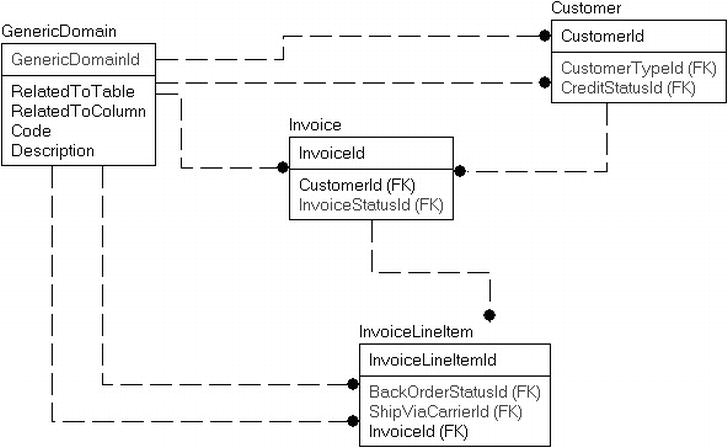
Figure 8-18. One multiuse domain table
I agree with you if you are thinking that this seems like a very clean way to implement this from a coding-only standpoint. The problem from a relational coding/implementation standpoint is that it is just not natural to work with in SQL. In many cases, the person who does this does not even think about SQL access. The data in GenericDomain is most likely read into cache in the application and never queried again. Unfortunately, however, this data will need to be used when the data is reported on. For example, say the report writer wants to get the domain values for the Customer table:
SELECT *
FROM Customer
JOIN GenericDomain as CustomerType
ON Customer.CustomerTypeId = CustomerType.GenericDomainId
AND CustomerType.RelatedToTable = 'Customer'
AND CustomerType.RelatedToColumn = 'CustomerTypeId'
JOIN GenericDomain as CreditStatus
ON Customer.CreditStatusId = CreditStatus.GenericDomainId
AND CreditStatus.RelatedToTable = 'Customer'
AND CreditStatus.RelatedToColumn = ' CreditStatusId'
As you can see, this is far from being a natural operation in SQL. It comes down to the problem of mixing apples with oranges. When you want to make apple pie, you have to strain out only apples so you don’t get them mixed. At first glance, domain tables are just an abstract concept of a container that holds text. And from an implementation-centric standpoint, this is quite true, but it is not the correct way to build a database because we never want to mix the rows together as the same thing ever in a query. The litmus test is if you will never use a domain except for one table, it should have its own table. You can tell this pretty easily usually, because you will need to specify a table and/or column name to figure out the rows that are applicable.
In a database, the process of normalization as a means of breaking down and isolating data takes every table to the point where one table represents one type of thing and one row represents the existence of one of those things. Every independent domain of values should be thought of as a distinctly different thing from all the other domains (unless it is not, in which case one table will suffice). So, what you do, in essence, is normalize the data over and over on each usage, spreading the work out over time, rather than doing the task once and getting it over with.
Instead of a single table for all domains, you should model it as shown in Figure 8-19.
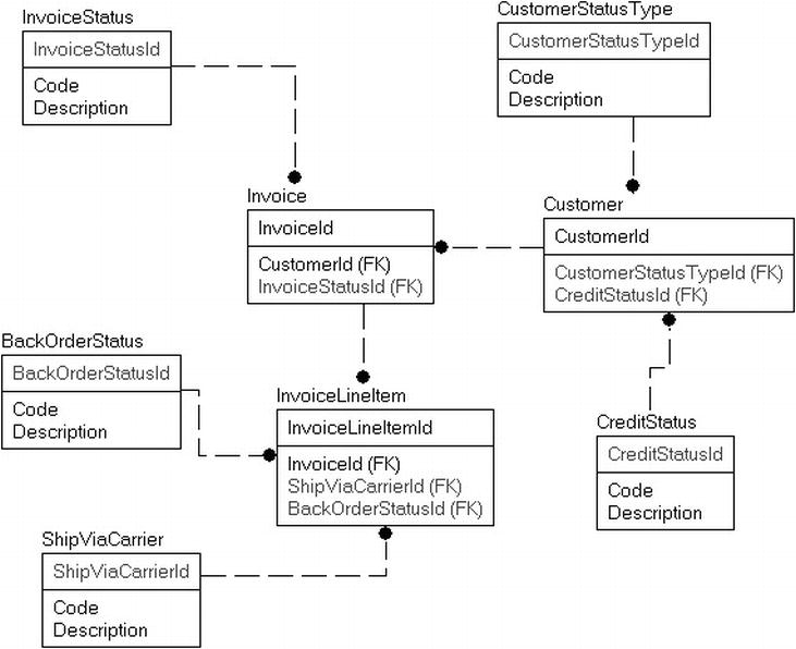
Figure 8-19. One domain table per purpose
That looks harder to do, right? Well, it is initially (like for the 5 or 10 minutes it takes to create a few tables). Frankly, it took me longer to flesh out the example tables. The fact is, there are quite a few tremendous gains to be had:
-
Using the data in a query
is much Clearer:
SELECT *
FROM Customer
JOIN CustomerType
ON Customer.CustomerTypeId = CustomerType.CustomerTypeId
JOIN CreditStatus
ON Customer.CreditStatusId = CreditStatus.CreditStatusId
- Data can be validated using simple foreign key constraints: This was something not feasible for the one-table solution. Now, validation needs to be in triggers or just managed solely by the application.
- Expandability and control: If it turns out that you need to keep more information in your domain row, it is as simple as adding a column or two. For example, if you have a domain of shipping carriers, you might define a ShipViaCarrier in your master domain table. In its basic form, you would get only one column for a value for the user to choose. But if you wanted to have more information—such as a long name for reports, as in “United Parcel Service”; a description; and some form of indication when to use this carrier—you would be forced to implement a table and change all the references to the domain values.
- Performance considerations: All of the smaller domain tables will fit on a single page or disk. This ensures a single read (and likely a single page in cache). If the other case, you might have your domain table spread across many pages, unless you cluster on the referring table name, which then could cause it to be more costly to use a nonclustered index if you have many values. In a very large table, it could get to the point where a scan of a larger domain table could get costly where only a very small number of rows is needed.
- You can still make the data look like one table for the application: There is nothing precluding developers from building a caching mechanism that melds together all the individual tables to populate the cache and use the data however they need it for the application. With some clever use of extended properties, this could be as simple as adding a value to a property and letting a dynamic SQL procedure return all the data. A common concern that developers have is that now they will need 50 editors instead of one. You can still have one editor for all rows, because most domain tables will likely have the same base structure/usage, and if they don’t, you will already need to create a new table or do some sort of hokey usage to make the single table design work.
Returning to the basics of design, every table should represent one and only one thing. When you see a column in a table by itself, there should be no question as to what it means, and you certainly shouldn’t need to go to the table and figure out what the meaning of a value is.
Some tools that implement an object-oriented view of a design tend to use this frequently, because it’s easy to implement tables such as this and use a cached object. One table means one set of methods instead of hundreds of different methods for hundreds of different objects—er, tables. (The fact that it stinks when you go to use it in the database for queries is of little consequence, because generally systems like this don’t, at least initially, intend for you to go into the database and do queries, except through special interfaces that take care of this situation for you.)
Generic Key References
In an ideal situation, one table is related to another via a key. However, because the structures in SQL Server don’t require constraints or any enforcement, this can lead to interesting relationships occurring. What I am referring to here is the case where you have a table that has a primary key that can actually be a value from several different tables, instead of just one.
For example, consider the case where you have several objects, all of which need a reference to one table. In our sample, say you have a customer relationship management system with SalesOrders and TroubleTickets (just these two to keep it simple, but in reality, you might have many objects in your database that will fit this scenario). Each of these objects has the need to store journal items, outlining the user’s contact with the customer (for example, in the case where you want to make sure not to overcommunicate with a customer!). You might logically draw it up like in Figure 8-20.
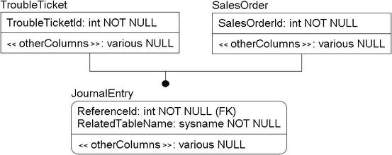
Figure 8-20. Multiple tables related to the same key
You might initially consider modeling it like a classic subtype relationship, but it really doesn’t fit that mold because you probably can have more than one journal entry per sales order and trouble ticket. Fair enough, each of these relationships is 1–N, where N is between 0 and infinity (though the customer with infinite journal entries must really hate you). Having all parents relate to the same column is a possible solution to the problem but not a very favorable one. For our table in this scenario, we build something like this:
CREATE TABLE SalesOrder
(
SalesOrderId <int or uniqueidentifier> PRIMARY KEY,
<other columns>
);
CREATE TABLE TroubleTicket
(
TroubleTicketId <int or uniqueidentifier> PRIMARY KEY,
<other columns>
);
CREATE TABLE JournalEntry
(
JournalEntryId <int or uniqueidentifier>,
RelatedTableName sysname,
PRIMARY KEY (JournalEntryId, RelatedTableName)
<other columns>
);
Now, to use this data, you have to indicate the table you want to join to, which is very much a unnatural way to do a join. You can use a universally unique GUID key so that all references to the data in the table are unique, eliminating the need for the specifically specified related table name. However, I find when this method is employed if the RelatedTableName is actually used, it is far clearer to the user what is happening.
A major concern with this method is that you cannot use constraints to enforce the relationships; you need either to use triggers or to trust the middle layers to validate data values, which definitely increases the costs of implementation/testing, since you have to verify that it works in all cases, which is something we trust for constraints; even triggers are implemented in one single location.
One reason this method is employed is that it is very easy to add references to the one table. You just put the key value and table name in there, and you are done. Unfortunately, for the people who have to use this for years and years to come, well, it would have just been easier to spend a bit longer and do some more work, because the generic relationship means that using a constraint is not possible to validate keys, leaving open the possibility of orphaned data.
A second way to do this that is marginally better is to just include keys from all tables, like this:
CREATE TABLE JournalEntry
(
JournalEntryId <int or uniqueidentifier> PRIMARY KEY,
SalesOrderId <int or uniqueidentifier> NULL REFERERENCES
SalesOrder(SalesOrderId),
TroubleTicketId <int or uniqueidentifier> NULL REFERERENCES
TroubleTicket(TroubleTicketId),
<other columns>
);
This is better, in that now joins are clearer and the values are enforced by constraints, but now, you have one more problem (that I conveniently left out of the initial description). What if you need to store some information about the reason for the journal entry? For example, for an order, are you commenting in the journal for a cancelation notice?
There is also the matter of nor concerns, since normalization/usage concerns in that the related values doesn’t exactly relate to the key in the same way. It seems like a decent idea that one JournalEntry might relate to more than one SalesOrder or JournalEntry. So, the better idea is to model it more like Figure 8-21.
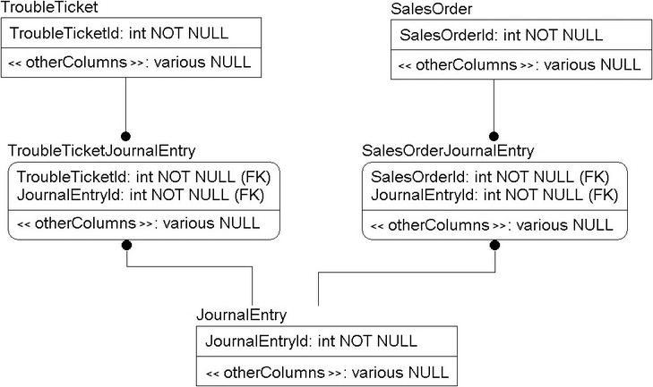
Figure 8-21. Objects linked for maximum usability/flexibility
CREATE TABLE JournalEntry
(
JournalEntryId <int or uniqueidentifier> PRIMARY KEY,
<other columns>
);
CREATE TABLE SalesOrderJournalEntry
(
JournalEntryId <int or uniqueidentifier>
REFERENCES JournalEntry(JournalId),
SalesOrderId <int or uniqueidentifier>,
REFERENCES SalesOrder(SalesOrderId),
<SalesOrderSpecificColumns>
PRIMARY KEY (JournalEntryId, SalesOrderId)
);
CREATE TABLE TroubleTicketJournalEntry
(
JournalEntryId <int or uniqueidentifier>
REFERENCES JournalEntry(JournalId),
TroubleTicketId <int or uniqueidentifier>,
REFERENCES TroubleTicket (TroubleTicketId),
<TroubleTicketSpecificColumns>
PRIMARY KEY (JournalEntryId, SalesOrderId)
);
Note that this database is far more self-documented as well. You can easily find the relationships between the tables and join on them. Yes, there are a few more tables, but that can play to your benefit as well in some scenarios, but most important, you can represent any data you need to represent, in any cardinality or combination of cardinalities needed. This is the goal in almost any design.
Overusing Unstructured Data
As much as I would like to deny it, or at least find some way to avoid it, people need to have unstructured notes to store various bits and pieces of information about their data. I will confess that a large number of the tables I have created in my career included some column that allowed users to insert whatever into. In the early days, it was a varchar(256) column, then varchar(8000) or text, and now varchar(max). It is not something that you can get away from, because users need this scratchpad just slightly more than Linus needs his security blanket. And it is not such a terrible practice, to be honest. What is the harm in letting the user have a place to note that the person has special requirements when you go out to lunch?
Nothing much, except that far too often what happens is that notes become a replacement for the types of stuff that I mentioned in the “User-Specified Data” section or, when this is a corporate application, the types of columns that you could go in and create in 10 minutes or about 2 days, including testing and deployment. Once the users do something once and particularly finds it useful, they will do it again. And they tell their buddies, “Hey, I have started using notes to indicate that the order needs processing. Saved me an hour yesterday .” Don’t get me wrong, I have nothing against users saving time, but in the end, everyone needs to work together.
See, if storing some value unstructured in a notes column saves the user any time at all (considering that, most likely, it will require a nonindexed search or a one-at-a-time manual search), just think what having a column in the database could do that can be easily manipulated, indexed, searched on, and oblivious to the spelling habits of the average human being. And what happens when a user decides that they can come up with a “better” way and practices change, or, worse, everyone has their own practices?
Probably the most common use of this I have seen that concerns me is contact notes. I have done this myself in the past, where you have a column that contains formatted text something like the following on a Customer table. Users can add new notes but usually are not allowed to go back and change the notes.
![]() ContactNotes 2008-01-11 – Stuart Pidd -Spoke to Fred on the phone. Said that his wangle was broken, referencing Invoice 20001. Told him I would check and call back tomorrow. 2008-02-15 – Stuart Pidd – Fred called back, stating his wangle was still broken, and now it had started to dangle. Will call back tomorrow. 2008-04-12 – Norm Oliser – Stu was fired for not taking care of one of our best customers.
ContactNotes 2008-01-11 – Stuart Pidd -Spoke to Fred on the phone. Said that his wangle was broken, referencing Invoice 20001. Told him I would check and call back tomorrow. 2008-02-15 – Stuart Pidd – Fred called back, stating his wangle was still broken, and now it had started to dangle. Will call back tomorrow. 2008-04-12 – Norm Oliser – Stu was fired for not taking care of one of our best customers.
What a terrible waste of data. The proper solution would be to take this data that is being stored into this text column and apply the rigors of normalization to it. Clearly, in this example, you can see three “rows” of data, with at least three “columns.” So instead of having a Customer table with a ContactNotes column, implement the tables like this:
CREATE TABLE Customer
(
CustomerId int CONSTRAINT PKCustomer PRIMARY KEY
<other columns>
);
CREATE TABLE CustomerContactNotes
(
CustomerId int,
NoteTime datetime,
PRIMARY KEY (CustomerId, NoteTime),
UserId datatype, --references the User table
Notes varchar(max)
);
You might even stretch this to the model we discussed earlier with the journal entries where the notes are a generic part of the system and can refer to the customer, multiple customers, and other objects in the database. This might even link to a reminder system to remind Stu to get back to Fred, and he would not now be jobless. Though one probably should have expected such out of a guy named Stu Pidd (ba boom ching).
Even using XML to store the notes in this structured manner would be an amazing improvement. You could then determine who entered the notes, what the day was, and what the notes were, and you could fashion a UI that allowed the users to add new fields to the XML, right on the fly. What a tremendous benefit to your users and, let’s face it, to the people who have to go in and answer questions like this, “How many times have we talked to this client by phone?”
The point of this section is simply this: educate your users. Give them a place to write the random note, but teach them that when they start to use notes to store the same specific sorts of things over and over, their jobs could be easier if you gave them a place to store their values that would be searchable, repeatable, and so on. Plus, never again would you have to write queries to “mine” information from notes.
![]() Tip SQL Server provides a tool to help search text called Full Text Search. It can be very useful for searching textual data in a manner much like a typical web search. However, it is no replacement for proper design that makes a different column and row from every single data point that the users are typically interested in.
Tip SQL Server provides a tool to help search text called Full Text Search. It can be very useful for searching textual data in a manner much like a typical web search. However, it is no replacement for proper design that makes a different column and row from every single data point that the users are typically interested in.
Summary
This chapter was dedicated to expanding the way you think about tables and to giving you some common solutions to problems that are themselves common. I was careful not to get too esoteric with my topics in this chapter. The point was simply to cover some solutions that are a bit beyond the basic table structures I covered in earlier chapters but not so beyond them that the average reader would say “Bah!” to the whole chapter as a waste of time.
The “good” patterns we covered were:
- Uniqueness: Simple uniqueness constraints are often not enough to specify uniqueness for “real” data. We discussed going deeper than basic implementation and working through uniqueness scenarios where you exclude values (selective uniqueness), bulk object uniqueness, and discussed the real-world example of trying to piece together uniqueness where you can’t be completely sure (like visitors to a web site).
- Data-driven design: The goal being to build your databases flexible enough that adding new data to the database that looks and acts like previous values does not require code changes. We do this by attempting to avoid hard-coded data that is apt to change and making columns for typical configurations.
- Hierarchies: We discussed several methods of implementing hierarchies, using simple SQL constructs to using hierarchyId, as well as an introduction to the different methods that have been created to optimize utilization with a bit of reduction in simplicity.
- Large binary data: This pertains particularly to images but could refer any sort of file that you might find in a Windows file system. Storing large binary values allows you to provide your users with a place to extend their data storage.
- Generalization: Although this is more a concept than a particular pattern, we discussed why we need to match the design to the users realistic needs by generalizing some objects to the system needs (and not to our nerdy academic desires).
We finished up with a section on anti-patterns and poor design practices, including some pretty heinous ones:
- Undecipherable data: All data in the database should have some sort of meaning. Users should not have to wonder what a value of 1 means.
- Overusing unstructured data: Basically, this hearkens back to normalization, where we desire to store one value per column. Users are given a generic column for notes regarding a given item, and because they have unplanned-for needs for additional data storage, they use the notes instead. The mess that ensues, particularly for the people who need to report onthis data, is generally the fault of the architect at design time to not give the users a place to enter whatever they need, or to be fair, the users changing their needs over time and adapting to the situation rather than consulting the IT team to adjust the system to their ever changing needs.
- One domain table to cover all domains: This is yet another normalization issue, because the overarching goal of a database is to match one table with one need. Domain values may seem like one thing, but the goal should be that every row in a table is usable in any table it is relatable to.
- Generic key references: It is a very common need to have multiple tables relate to another. It can also be true that only one table should be related at a time. However, every column should contain one and only one type of data. Otherwise, users have no idea what a value is unless they go hunting.
Of course, these lists are not exhaustive of all of the possible patterns out there that you should use or not use, respectively. The goal of this chapter was to help you see some of the common usages of objects so you can begin to put together models that follow a common pattern where it makes sense. Feedback, particularly ideas for new sections, is always desired at [email protected].