
![]()
People use reporting in every aspect of their daily lives. Reports provide the local weather, the status of the morning train, and even the best place to get a cup of joe. And this is all before getting to work! At work, reports include enterprise dashboards, system outage reports, and timesheet cards. Any way you slice it, reporting is something that no one can get away from.
Wouldn’t it be nice if you could understand how that reporting works? How the reports get put together and how the information is stored underneath the covers? This chapter will show you how that happens, by discussing two types of reporting you may encounter: analytical and aggregation. You will learn more about each area, including the types of dimensional modeling and how to get started on your own dimensional model. You will also create an aggregation model. Finally, you will look at common queries that can be used to retrieve information from each of these models.
Keep in mind that there are entire sets of books dedicated just to reporting, so you won’t learn everything here, but hopefully, you’ll learn enough to get you started on your own reporting solution.
Reporting can mean different things to different people and can be used in different ways. Reporting can lean toward the analytical, or even be used as an aggregation engine to display a specific set of information. Although each of these purposes is a valid reporting option, each has a unique way of storing information to ensure it can quickly and accurately satisfy its purpose and provide the correct information.
I’ve often had the debate with coworkers, clients, and friends of the best way to store data in a database. While methodologies differ, the overarching viewpoints revolve around two focuses: data in and data out. Or as Claudia Imhoff has stated in “Are You an Inny or an Outty?” ( http://www.information-management.com/issues/19990901/1372-1.html ). Innies are people who are most interested in storing the data into the table in the most efficient and quick way. On the other hand, outties are those who are most interested in making the output of the data as simple as possible for the end user. Both types of people can be involved in relational or data warehouse design. I unabashedly admit to being an outty. My entire goal of storing data is to make it easier for someone to get it out. I don’t care if I need to repeat values, break normalization practices, or create descriptive column names that could compete with an anaconda for length.
The reporting styles that I utilize to handle these reporting situations that are discussed in this chapter are:
Each modeling paradigm has its own particular way of modeling the underlying database and storing the data. We will dig further into each of these reporting styles in this chapter.
Probably the best-known method for storing data for analytical reporting is a dimensional model. Analytics focuses on two areas: understanding what happened and forecasting or trending what will happen. Both of these areas and questions can be solved using a dimensional model.
Dimensional modeling is a very business focused type of modeling. Knowing the business process of how the data is used is important in being able to model it correctly. The same set of information can actually be modeled in two different ways, based on how the information is used! In the database modeling technique of dimensional modeling, denormalization is a good thing. You will see how to create a dimensional model later in this chapter.
Dimensional models are typically used in data warehouses or datamarts. There are two leading methodologies for creating a dimensional model, led by two amazing technologists: Ralph Kimball and Bill Inmon. There are others as well, but we will focus on these two methodologies. While I typically use an approach more like Kimball’s, both methodologies have benefits and can be used to create a successful dimensional model and analytical reporting solution.
Ralph Kimball
Ralph Kimball’s approach to data warehousing and dimensional modeling is typically known as a bottom-up approach. This name signifies a bus architecture, in which a number of datamarts are combined using similar dimensions to create an enterprise data warehouse. Each data mart (and in turn, the data warehouse) is created used a star or snowflake schema, which contains one or more fact tables, linked to many dimensions.
To create the bus architecture, datamarts are created that are subject oriented and contain business logic for a particular department. Over time, new datamarts are created, using some of the same entities or dimensions as the original datamart. Eventually, the datamarts grow to create a full enterprise data warehouse.
For more information on Ralph Kimball’s approach, see http://www.kimballgroup.com .
The other leading data warehouse methodology is proponed by Bill Inmon and is typically known as a top-down approach. In this scenario, “top-down” means starting with an enterprise warehouse and creating subject area datamarts from that data warehouse. The enterprise data warehouse is typically in a third-normal form, which was covered in Chapter 5, while data marts are typically in a dimensional format.
Inmon also created the concept of a corporate information factory, which combines all organization systems, including applications and data storage, into one cohesive machine. Operational data stores, enterprise data warehouses, and data management systems are prevalent in these systems.
See http://www.inmoncif.com for additional information on Bill Inmon’s approach.
A hybrid of analytical and relational reporting, aggregation reporting combines the best of both worlds to create a high-performing set of information in specific reporting scenarios. This information is used for some analysis and is also used operationally. By creating a set of aggregated values, report writers can quickly pull exactly the information they need.
Modeling summary tables typically occurs when a report that used an aggregated value becomes too slow for the end users. This could be because the amount of data that was aggregated has increased or the end users are doing something that wasn’t originally planned for. To fix the slow reporting situation, summary tables can be created to speed up the reports without having to create a whole data warehouse.
Some scenarios where it may make sense to create summary tables include rolling up data over time and looking at departments or groups within a company where you can report on multiple levels. Aggregation reporting is especially useful when there is a separate reporting database where its resources can be consumed by queries and reports.
Requirements-Gathering Process
Before starting to do any modeling, it is essential to gather the requirements for the end solution. In this case, the word “requirements” doesn’t mean how the end solution should look or who should have access to it. “Requirements” refers to who will use information and how they use it, particularly the business processes and results of using the data.
By talking to numerous members of the business, executive team, and key stakeholders, you will learn how the business works and what is valued. The corporate strategy and goals provide an important aspect to your requirements. They will ensure you are on the same page as the company and that your analytics can contribute to the high-level goals of the organization. At this time, I like to review the existing technical processes and data model. Because you understand the business inside and out, you will be able to see how the current infrastructure does or does not support the business.
Here, my system for gathering requirements veers off from typical processes. I like to create the initial data model as part of the requirements process. I find that I dig more deeply into understanding the relationship between entities, attributes, and processes if I am trying to put it into a data model. Then, if I can explain the data model in terms of a business process to the business folk, I am golden!
A recap of the steps listed in this section is shown in Figure 14-1.
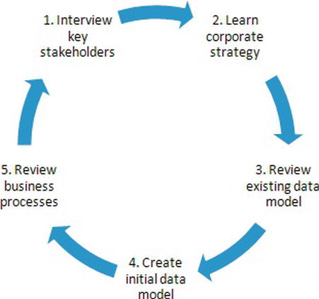
Figure 14-1. Requirements gathering steps diagram
Whether you require an analytical or aggregation reporting solution, you will still follow a similar requirements process. The process that ports the business process requirements into a particular type of data model (described as step 4) will be described in the following sections of this chapter.
The requirements-gathering phase is a very important step in any software development life cycle, including a reporting solution. Be firm about talking to the business as well as the technology department.
At the end of a business intelligence project, I often find myself in a situation where I am explaining a piece of the business to someone from another department. Because of the perpetual silos that occur in a company, it’s too easy to ignore something that doesn’t affect you directly. Your goal as a reporting modeler is to learn about all areas and processes. Often, you’ll discover ties between the siloed departments that were impossible to initially see!
Dimensional Modeling for Analytical Reporting
The design principles in this section describe dimensional modeling, which is used for analytical reporting. Dimensional modeling takes a business process and separates it into logical units, typically described as entities, attributes, and metrics. These logical units are split into separate tables, called dimensions and facts. Additional tables can be included, but these are the two most common and important tables that are used.
Following are the different types of tables we will work with in a dimensional model:
- Dimension: A dimension table contains information about an entity. All descriptors of that entity are included in the dimension. The most common dimension is the date dimension, where the entity is a day and the descriptors include month, year, and day of week.
- Fact: A fact table is the intersection of all of the dimensions and includes the numbers you care about, also known as measures. The measures are usually aggregatable, so they can be summed, averaged, or used in calculations. An example of a fact table would be a store sales fact, where the measures include a dollar amount and unit quantity.
- Bridge: A bridge table, also known as a many-to-many table, links two tables together that cannot be linked by a single key. There are multiple ways of presenting this bridge, but the outcome is to create a many-to-many relationship between two dimensions tables.
We will start by describing the different types of dimensions that you can create and wrap up with the types of facts you can create. After we complete our discussion of facts and dimensions, we will end up with a complete health care insurer data model, as shown in Figure 14-2.
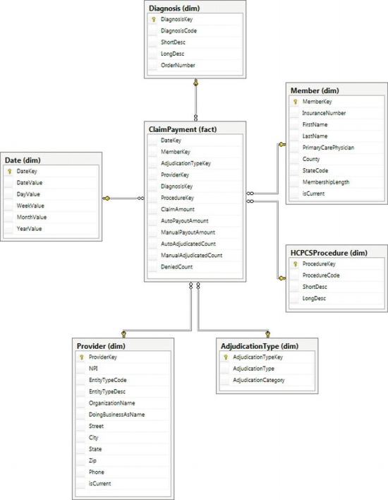
Figure 14-2. Completed health care payer dimensional model
As previously stated, a dimension is the table that describes an entity. Once the business process is described, the first step is to determine what dimensions we need. Then, we can decide on what type of dimension we need to use, what the grain (or smallest detail) of the dimension should be, and finally, what we want to put into the dimension. Let’s start with business process.
While the claim payment business process is fairly complicated, we will use a limited version to illustrate a dimensional model. When an insurance company receives a claim for a member, the claim goes through an adjudication process. The claim can either be automatically adjudicated, manually adjudicated, or denied. As an insurance company, we need to know whether we adjudicated the claim, how much the physician requested based on the member’s diagnosis, and how much we are willing to pay for that procedure.
Sometimes, translation between the technical and business folks can be difficult, so try to understand how the business works and talk in their language. Don’t try to relate the business to another field, and don’t assume that you understand what they are saying. Ask the questions in different ways and try to come up with edge cases to see if they may help you gain a deeper understanding. If 99 percent of camouflage pants come in green or gray, but 1 percent comes in purple, you must know about that 1 percent from a data perspective.
Once you’ve thought through the business process, it is easy to pick out the key entities. While getting started, it may help to write down the business as in the previous paragraph and then highlight the entities as you come to them. The following paragraph illustrates how to highlight the entities from the business process:
When an insurance company receives a claim for a member, the claim goes through an adjudication process . The claim can either be automatically adjudicated, manually adjudicated, or denied. As an insurance company, we need to know whether we adjudicated the claim, how much the physician requested based on the member’s diagnosis, and how much we are willing to pay for that procedure.
Using those italicized phrases, our dimensions are: date, member, adjudication type, physician/provider, diagnosis, and procedure. Once we have the dimensions, it is important to talk to the business to find out what the grain for each of those dimensions should be. Do we receive claims on a daily or monthly basis? Is a member defined as an insurance number, a social security number, or a household? And so on. These are questions that must be asked of and answered by the business.
You must know where the data will be sourced from to ensure that the correct names and datatypes are used in the model. Fortunately, healthcare is a field that has standard definitions and files for many of the entities that we are interested in! During the walkthrough of each entity, any standard sources will be called out.
Once you have gone through the requirements process, discovered all of the business processes, and know everything there is to know about your business, it is time to start modeling! I like to start with dimensions, as the facts seem to fall into place after that. If you recall from earlier in the chapter, a dimension is an entity and its descriptors. Dimensions also include hierarchies, which are levels of properties that relate to each other in groups. Let’s walk through a few examples of dimensions to solidify everything we’ve discussed.
The date dimension is the most common dimension, as almost every business wants to see how things change over time. Sometimes, the business even wants to see information at a lower granularity than date, such as at an hour or minute level. While it is tempting to combine the time granularity with the date dimension, don’t do it! Analysis is typically done at either the time or date level, so a rollup is not necessary, and you will inflate the number of rows in your dimension (365 days * 1440 minutes = 525,600 rows in your table). Let’s walk through the thought process of creating the date dimension, and then, you can use a similar thought process to create a separate time dimension.
You can always start with a base date dimension and modify it to suit your needs. The base date dimension should have the following features:
- An integer key that uniquely identifies that row: Sometimes, a surrogate key is used, which has absolutely no business value and can be implemented using an IDENTITY column. My recommendation is to use a smart key, which combines the year and date in an eight-digit number, such as 20110928, for September 28, 2011 for the United States folks. Smart keys make sense for date and time dimensions, because you know the entity itself will never change. In other words, September 28, 2011 will always be in the month of September and will always be in the year 2011.
- The business key that represents the entity : For a date dimension, this value is very simple; it is just the date. This business key should always be the lowest granularity of information stored in your dimension.
- Additional standard attributes : These attributes can include information about whether this date is a holiday, whether a promotion is running during this time, or additional fields describing a fiscal calendar
The code to create a base date dimension table is listed here:
-- Create schema for all dimension tables
CREATE SCHEMA dim
GO
-- Create Date Dimension
CREATE TABLE dim.Date
(
DateKey INTEGER NOT NULL,
DateValue DATE NOT NULL,
DayValue INTEGER NOT NULL,
WeekValue INTEGER NOT NULL,
MonthValue INTEGER NOT NULL,
YearValue INTEGER NOT NULL
CONSTRAINT PK_Date PRIMARY KEY CLUSTERED
(
DateKey ASC
))
GO
![]() Note When I create my table and column names, I use a particular naming convention that includes schemas to describe the table type, capital letters for each word in the name, and a set of suffixes that describe the column type. While this standard works for me, you should use a convention that fits into your organization’s standards.
Note When I create my table and column names, I use a particular naming convention that includes schemas to describe the table type, capital letters for each word in the name, and a set of suffixes that describe the column type. While this standard works for me, you should use a convention that fits into your organization’s standards.
To populate the dimension, you can use a stored procedure or script that will automatically add additional days as needed. Such a stored procedure follows. Note the initial insert statement that adds the unknown row if it doesn’t exist.
Unknown rows are used to symbolize that the relationship between a metric and a particular dimension entity does not exist. The relationship may not exist for a number of reasons:
- The relationship does not exist in the business process.
- The incoming feed does not yet know what the relationship should be.
- The information does not appear to be valid or applicable to the scenario.
By tying the fact table to the unknown row, it is very simple to see where the relationship is missing. The surrogate key for each unknown row is –1, and the descriptors contain variations of “unknown,” such as UN, -1, and UNK. Each dimension that we will create will contain an unknown row to highlight this use case.
In some cases, it may make sense to create multiple unknown rows to distinguish between the three reasons for having an unknown row. One reason why you may want to do this is if you have many late-arriving dimensions, where you are very concerned with the rows that have not yet been linked to a dimension. Another reason you may want to do this is if you have poor data quality, and it is important to distinguish between acceptable and unacceptable unknown rows.
The following stored procedure uses only one unknown row:
-- Create Date Dimension Load Stored Precedure
CREATE PROCEDURE dim.LoadDate (@startDate DATETIME, @endDate DATETIME)
AS
BEGIN
IF NOT EXISTS (SELECT * FROM dim.Date WHERE DateKey = -1)
BEGIN
INSERT INTO dim.Date
SELECT -1, '01/01/1900', -1, -1, -1, -1
END
WHILE @startdate <= @enddate
BEGIN
IF NOT EXISTS (SELECT * FROM dim.Date WHERE DateValue = @startdate)
INSERT INTO dim.Date
SELECT CONVERT(CHAR(8), @startdate, 112) AS DateKey
,@startdate AS DateValue
,DAY(@startdate) AS DayValue
,DATEPART(wk, @startdate) AS WeekValue
,MONTH(@startdate) AS MonthValue
,YEAR(@startdate) AS YearValue
SET @startdate = DATEADD(dd, 1, @startdate)
END
END
GO
The outcome of this stored procedure is to load any date values that are not yet in the date dimension. Running the following query will insert two years of date:
EXECUTE dim.LoadDate '01/01/2011', '12/31/2012'
GO
A sample of the data in the table is shown here:
|
DateKey |
DateValue |
DayValue |
WeekValue |
MonthValue |
YearValue |
|
-------- |
---------- |
-------- |
--------- |
---------- |
--------- |
|
-1 |
1900-01-01 |
-1 |
-1 |
-1 |
-1 |
|
20111230 |
2011-12-30 |
30 |
53 |
12 |
2011 |
|
20111231 |
2011-12-31 |
31 |
53 |
12 |
2011 |
|
20120101 |
2012-01-01 |
1 |
1 |
1 |
2012 |
|
20120102 |
2012-01-02 |
2 |
1 |
1 |
2012 |
This dimension and stored procedure may be exactly what you need, and if so, move onto the next section on slowly changing dimensions. On the other hand, there’s a good chance that you’ll need to go further with this dimension. To start, many organizations have fiscal calendars. You will use the same base date dimension, but add additional columns for FiscalDayValue, FiscalWeekValue, and so on. Along the same vein, you may also have date-specific descriptors that should be included. These could be as simple as calling out the federal holidays or as complicated as highlighting the various sales periods throughout the year. To include any of those additional items, you’ll want to modify the stored procedure to use the logic specific to your organization.
The date dimension is about as simple as a dimension can get. The information can be populated once or over time and is never modified. The rest of the dimensions won’t be that simple. To begin, we need to discuss the concept of slowly changing dimensions. Here are the most common types of slowly changing dimensions:
- Type 1, or changing: A type 1 change overwrites the value that was previously assigned to that attribute. A type 1 change is typically used when keeping the original value is not important. Example attributes include product category and company name.
- Type 2, or historical: A type 2 change is more in-depth than a type 1 change. It tracks any changes that occurred to that attribute over time so seeing the original, final, and any intermediate values is possible. Example historical attributes in which you may be interested include customer state and employee manager.
- Type 3, or hybrid: Finally, a type 3 change is a hybrid of both the type 1 and type 2 changes. It keeps track of the intermediate and final values on every row. This allows reporting to compare the current value with the latest value for any intermediate value or to be able to see the alternate view, as though the change didn’t happen. This approach is not often used, but one good example is comparing the average temperature for a location at that time versus the final average temperature over the life of the warehouse.
As this book has hammered over and over again, uniqueness is so very important when dealing with data. And I’m not going to contradict that now, except to say that it is possibly even more important when dealing with reporting. You need to determine the unique identifier, also known as the business key, for each entity. This key is how you will know how to link a dimension to a fact and how to create additional rows in the case of a slowly changing dimension.
In the case of a health insurance company, a member can change personal information on a regular basis, and seeing how that information tracks over time may be important. Let’s walk through the steps of creating the member dimension.
As with every dimension, we begin by determining the business key for the entity. For an insured member, the business key is the insurance number. Additional attributes for personal information that are analyzed include first name, last name, primary care physician, county, state, and membership duration. Our initial dimension can be created using the following script:
-- Create the Member dimension table
CREATE TABLE dim.Member
(
MemberKey INTEGER NOT NULL IDENTITY(1,1),
InsuranceNumber VARCHAR(12) NOT NULL,
FirstName VARCHAR(50) NOT NULL,
LastName VARCHAR(50) NOT NULL,
PrimaryCarePhysician VARCHAR(100) NOT NULL,
County VARCHAR(40) NOT NULL,
StateCode CHAR(2) NOT NULL,
MembershipLength VARCHAR(15) NOT NULL
CONSTRAINT PK_Member PRIMARY KEY CLUSTERED
(
MemberKey ASC
))
GO
For demonstration’s sake, load the member dimension with the following INSERT script:
-- Load Member dimension table
SET IDENTITY_INSERT [dim].[Member] ON
GO
INSERT INTO [dim].[Member]
([MemberKey],[InsuranceNumber],[FirstName],[LastName],[PrimaryCarePhysician]
,[County],[StateCode],[MembershipLength])
VALUES
(-1, 'UNKNOWN','UNKNOWN','UNKNOWN','UNKNOWN','UNKNOWN','UN','UNKNOWN')
GO
SET IDENTITY_INSERT [dim].[Member] OFF
GO
INSERT INTO [dim].[Member]
([InsuranceNumber],[FirstName],[LastName],[PrimaryCarePhysician]
,[County],[StateCode],[MembershipLength])
VALUES
('IN438973','Brandi','Jones','Dr. Keiser & Associates','Henrico','VA','<1 year')
GO
INSERT INTO [dim].[Member]
([InsuranceNumber],[FirstName],[LastName],[PrimaryCarePhysician]
,[County],[StateCode],[MembershipLength])
VALUES
('IN958394','Neil','Gomez','Healthy Lifestyles','Henrico','VA','1-2 year')
GO
INSERT INTO [dim].[Member]
([InsuranceNumber],[FirstName],[LastName],[PrimaryCarePhysician]
,[County],[StateCode],[MembershipLength])
VALUES
('IN3867910','Catherine','Patten','Dr. Jenny Stevens','Spotsylvania','VA','<1 year')
GO
Use the following query to retrieve the sample data that follows:
select MemberKey, InsuranceNumber, FirstName, LastName, PrimaryCarePhysician
from dim.Member
GO
Here are the results:
|
MemberKey |
Insurance |
FirstName |
LastName |
PrimaryCarePhysician |
|
----------- |
----------- |
----------- |
---------- |
--------------------- |
|
-1 |
UNKNOWN |
UNKNOWN |
UNKNOWN |
UNKNOWN |
|
1 |
IN438973 |
Brandi |
Jones |
Dr. Keiser & Associates |
|
2 |
IN958394 |
Neil |
Gomez |
Healthy Lifestyles |
|
3 |
IN3867910 |
Catherine |
Patten |
Dr. Jenny Stevens |
What do we do when a piece of information changes? Well, if it’s something that we want to track, we use a type 2 change. If it’s something we don’t care about, we use type 1. We must know which type we want to track at modeling time to make some adjustments. In the case of the member dimension, we want to use a type 2 attribute. We know this because we want to track if a member’s primary care physician (PCP) changes to verify that we are only paying out for visits to a PCP. To track this information as the type 2 attribute, we need to add a flag called isCurrent to indicate which row contains the most current information. The code to add this field is listed here:
ALTER TABLE dim.Member
ADD isCurrent INTEGER NOT NULL DEFAULT 1
GO
When a load process runs to update the member dimension, it will check to see if there is a match on the business key of InsuranceNumber, and if so, it will add an additional row but flip the isCurrent bit on the old row to 0. Use the following code to emulate Brandi changing her primary care physician and updating the old record:
INSERT INTO [dim].[Member]
([InsuranceNumber],[FirstName],[LastName],[PrimaryCarePhysician]
,[County],[StateCode],[MembershipLength])
VALUES
('IN438973','Brandi','Jones','Dr. Jenny Stevens','Henrico','VA','<1 year')
GO
UPDATE [dim].[Member] SET isCurrent = 0
WHERE InsuranceNumber = 'IN438973' AND PrimaryCarePhysician = 'Dr. Keiser & Associates'
GO
If we use a similar query as before, but add the new isCurrent column as follows, we see the full change of the dimension:
select MemberKey, InsuranceNumber, FirstName, LastName, PrimaryCarePhysician, isCurrent
from dim.Member
And here are the results:
|
MemberKey |
Insurance |
FirstName |
LastName |
PrimaryCarePhysician |
isCurrent |
|
--------- |
--------- |
--------- |
-------- |
----------------------- |
--------- |
|
-1 |
UNKNOWN |
UNKNOWN |
UNKNOWN |
UNKNOWN |
1 |
|
1 |
IN438973 |
Brandi |
Jones |
Dr. Keiser & Associates |
0 |
|
2 |
IN958394 |
Neil |
Gomez |
Healthy Lifestyles |
1 |
|
3 |
IN3867910 |
Catherine |
Patten |
Dr. Jenny Stevens |
1 |
|
4 |
IN438973 |
Brandi |
Jones |
Dr. Jenny Stevens |
1 |
![]() Note For a more detailed explanation of how to programmatically add the logic for a type 2 dimension using SSIS, see Apress’s Pro SQL Server 2012 Integration Services by Michael Coles and Francis Rodrigues.
Note For a more detailed explanation of how to programmatically add the logic for a type 2 dimension using SSIS, see Apress’s Pro SQL Server 2012 Integration Services by Michael Coles and Francis Rodrigues.
An alternative to using the isCurrent flag is to use two columns: start date and end date. The start date describes when the row first became active, and the end date is when that row has expired. If the row has not yet expired, the value is null. If you wanted to see all current values, you can query all rows where the end date is null. In addition to that information, you can also see when each dimension row changed without having to look at the fact table.
You may ask yourself why you need any flag or date range. Isn’t it possible to just find the latest row based on the growing identity key, where the maximum value is the current one? You would be absolutely correct that you can get the same information; however, the query to pull that information is more complicated and difficult to pull. As a case in point, would you rather write the query in Listing 14-1 or 14-2 on a regular basis?
Listing 14-1. Preferred Query to Pull the Latest Dimension Row
select * from dim.Member where isCurrent = 1
GO
Listing 14-2. Rejected Query to Pull the Latest Dimension Row
select * from (
select m.*, ROW_NUMBER() OVER (PARTITION BY m.InsuranceNumber
ORDER BY m.MemberKey DESC) As Latest
from dim.Member m ) LatestMembers
WHERE LatestMembers.Latest = 1
GO
The provider dimension is similar to the member dimension, as it can change over time. The information in this information is based on a standard through the National Provider Registry, which can be found at http://www.cms.gov/NationalProvIdentStand/downloads/Data_Dissemination_File-Readme.pdf . By using a limited set of information, we can create a dimension as described here:
-- Create the Provider dimension table
CREATE TABLE dim.Provider (
ProviderKey INTEGER IDENTITY(1,1) NOT NULL,
NPI VARCHAR(10) NOT NULL,
EntityTypeCode INTEGER NOT NULL,
EntityTypeDesc VARCHAR(12) NOT NULL, -- (1:Individual,2:Organization)
OrganizationName VARCHAR(70) NOT NULL,
DoingBusinessAsName VARCHAR(70) NOT NULL,
Street VARCHAR(55) NOT NULL,
City VARCHAR(40) NOT NULL,
State VARCHAR(40) NOT NULL,
Zip VARCHAR(20) NOT NULL,
Phone VARCHAR(20) NOT NULL,
isCurrent INTEGER NOT NULL DEFAULT 1
CONSTRAINT PK_Provider PRIMARY KEY CLUSTERED
(
ProviderKey ASC
))
GO
Add an initial set of data using the following query:
-- Insert sample data into Provider dimension table
SET IDENTITY_INSERT [dim].[Provider] ON
GO
INSERT INTO [dim].[Provider]
([ProviderKey],[NPI],[EntityTypeCode],[EntityTypeDesc],[OrganizationName],
[DoingBusinessAsName],[Street],[City],[State],[Zip],[Phone])
VALUES
(-1, 'UNKNOWN',-1,'UNKNOWN','UNKNOWN','UNKNOWN','UNKNOWN','UNKNOWN','UNKNOWN','UNKNOWN','UNKNOWN')
GO
SET IDENTITY_INSERT [dim].[Provider] OFF
GO
INSERT INTO [dim].[Provider]
([NPI],[EntityTypeCode],[EntityTypeDesc],[OrganizationName],
[DoingBusinessAsName],[Street],[City],[State],[Zip],[Phone])
VALUES
('1234567',1,'Individual','Patrick Lyons','Patrick Lyons','80 Park St.',
'Boston','Massachusetts','55555','555-123-1234')
GO
INSERT INTO [dim].[Provider]
([NPI],[EntityTypeCode],[EntityTypeDesc],[OrganizationName],
[DoingBusinessAsName],[Street],[City],[State],[Zip],[Phone])
VALUES
('2345678',1,'Individual','Lianna White, LLC','Dr. White & Associates','74 West Pine Ave.',
'Waltham','Massachusetts','55542','555-123-0012')
GO
INSERT INTO [dim].[Provider]
([NPI],[EntityTypeCode],[EntityTypeDesc],[OrganizationName],
[DoingBusinessAsName],[Street],[City],[State],[Zip],[Phone])
VALUES
('76543210',2,'Organization','Doctors Conglomerate, Inc','Family Doctors','25 Main Street Suite 108',
'Boston','Massachusetts','55555','555-321-4321')
GO
INSERT INTO [dim].[Provider]
([NPI],[EntityTypeCode],[EntityTypeDesc],[OrganizationName],
[DoingBusinessAsName],[Street],[City],[State],[Zip],[Phone])
VALUES
('3456789',1,'Individual','Dr. Drew Adams','Dr. Drew Adams','1207 Corporate Center',
'Peabody','Massachusetts','55554','555-234-1234')
GO
A dimension can have attributes of multiple types, so the last name can be type 1 while the primary care physician is type 2. I’ve never understood why they’re called slowly changing dimensions when they exist at an attribute level, but that’s the way it is.
In our discussion of modeling methodologies, we talked about star schemas and snowflake schemas. The key differentiator between those two methodologies is the snowflake dimension. A snowflake dimension takes the information from one dimension and splits it into two dimensions. The second dimension contains a subset of information from the first dimension and is linked to the first dimension, rather than the fact, through a surrogate key.
A great example of this is when one entity can be broken into two subentities that change on their own. By grouping the subentities’ properties together in their own dimension, they can change on their own or be linked directly to the fact on its own, instead of using the intermediary dimension, if the grain applies. However, breaking out an entity into a snowflake dimension is not without its downfalls. Never, ever, ever link both the first and second dimension to the same fact table. You’d create a circular relationship that could potentially cause discrepancies if your loads are not kept up to date. I also recommend never snowflaking your dimensions to more than one level, if at all. The added complexity and maintenance needed to support such a structure is often not worthwhile when alternative methods can be found. Let’s talk through a possible snowflake dimension, when you would want to use it, and alternative methods.
To continue our healthcare example, we will look at the types of insurance coverage provided by the company. There are multiple types of plans that each contains a set of benefits. Sometimes, we look at the metrics at the benefit level and other times, at the plan level. Even though we sometimes look at benefits and plans differently, there is a direct relationship between them.
Let’s begin by looking at each of the tables separately. The benefit table creation script is listed here:
-- Create the Benefit dimension table
CREATE TABLE dim.Benefit(
BenefitKey INTEGER IDENTITY(1,1) NOT NULL,
BenefitCode INTEGER NOT NULL,
BenefitName VARCHAR(35) NOT NULL,
BenefitSubtype VARCHAR(20) NOT NULL,
BenefitType VARCHAR(20) NOT NULL
CONSTRAINT PK_Benefit PRIMARY KEY CLUSTERED
(
BenefitKey ASC
))
GO
The health plan creation script is shown here:
-- Create the Health Plan dimension table
CREATE TABLE dim.HealthPlan(
HealthPlanKey INTEGER IDENTITY(1,1) NOT NULL,
HealthPlanIdentifier CHAR(4) NOT NULL,
HealthPlanName VARCHAR(35) NOT NULL
CONSTRAINT PK_HealthPlan PRIMARY KEY CLUSTERED
(
HealthPlanKey ASC
))
GO
I’ve already explained that a set of benefits can be tied to a plan, so we need to add a key from the benefit dimension to the plan dimension. Use an ALTER statement to do this, as shown:
ALTER TABLE dim.Benefit
ADD HealthPlanKey INTEGER
GO
ALTER TABLE dim.Benefit WITH CHECK
ADD CONSTRAINT FK_Benefit_HealthPlan
FOREIGN KEY(HealthPlanKey) REFERENCES dim.HealthPlan (HealthPlanKey)
GO
When the benefit key is added to a fact, the plan key does not also need to be added but will still be linked and can be used to aggregate or filter the information. In addition, if the grain of one of the fact tables is only at the plan level, the plan key can be used directly without having to use the benefit key.
We will not use the Benefit dimension in our model, but we will use the HealthPlan dimension. You can populate the data using the following script:
-- Insert sample data into Health plan dimension
INSERT INTO [dim].[HealthPlan]
([HealthPlanIdentifier],[HealthPlanName])
VALUES ('BRON','Bronze Plan')
GO
INSERT INTO [dim].[HealthPlan]
([HealthPlanIdentifier],[HealthPlanName])
VALUES ('SILV','Silver Plan')
GO
INSERT INTO [dim].[HealthPlan]
([HealthPlanIdentifier],[HealthPlanName])
VALUES ('GOLD','Gold Plan')
GO
An important concept that we have not yet covered is how to handle hierarchies in your data structure. Hierarchies are an important concept that you will hear about over and over again. Each level of the hierarchy is included in the same dimension, and the value of each parent level is repeated for every child value. In the Benefit dimension, BenefitSubtype and BenefitType create a hierarchy. Ensure that all subtypes have the same type in the load process to help later reporting.
Another common dimension type that often appears is what I like to call a type dimension, because it is often simple to identify due to its name. This dimension is a very simple one that typically contains a few type 1 changing attributes. Not all entities have to contain the word “type,” but it’s a nice indicator. Examples include transaction type, location type, and sale type.
In our health care example, the adjudication type is a perfect example of this dimension. The adjudication type dimension contains two columns and four rows, and the full creation script is shown here:
-- Create the AdjudicationType dimension table
CREATE TABLE dim.AdjudicationType (
AdjudicationTypeKey INTEGER IDENTITY(1,1) NOT NULL,
AdjudicationType VARCHAR(6) NOT NULL,
AdjudicationCategory VARCHAR(8) NOT NULL
CONSTRAINT PK_AdjudicationType PRIMARY KEY CLUSTERED
(
AdjudicationTypeKey ASC
))
GO
The values for the adjudication type dimension are static, so they can be loaded once, instead of on a recurring or nightly basis. The following INSERT script will insert the three business value rows and the one unknown row:
-- Insert values for the AdjudicationType dimension
SET IDENTITY_INSERT dim.AdjudicationType ON
GO
INSERT INTO dim.AdjudicationType
(AdjudicationTypeKey, AdjudicationType, AdjudicationCategory)
VALUES (-1, 'UNKNWN', 'UNKNOWN')
INSERT INTO dim.AdjudicationType
(AdjudicationTypeKey, AdjudicationType, AdjudicationCategory)
VALUES (1, 'AUTO', 'ACCEPTED')
INSERT INTO dim.AdjudicationType
(AdjudicationTypeKey, AdjudicationType, AdjudicationCategory)
VALUES (2, 'MANUAL', 'ACCEPTED')
INSERT INTO dim.AdjudicationType
(AdjudicationTypeKey, AdjudicationType, AdjudicationCategory)
VALUES (3, 'DENIED', 'DENIED')
GO
SET IDENTITY_INSERT dim.AdjudicationType OFF
GO
The values in this table can then be shown as follows:
|
AdjudicationTypeKey |
AdjudicationType |
AdjudicationCategory |
|
------------------- |
---------------- |
------------------- |
|
-1 |
UNKNWN |
UNKNOWN |
|
1 |
AUTO |
ACCEPTED |
|
2 |
MANUAL |
ACCEPTED |
|
3 |
DENIED |
DENIED |
This provides an easy way to filter any claim that you have on either the actual type of adjudication that occurred or the higher-level category.
Our final two dimensions also fit into this category: Diagnosis and HCPCSProcedure. Diagnosis and procedure codes contain a standard set of data fields. Diagnoses and procedure codes are known as International Classification of Diseases, Tenth Revision, Clinical Modification (ICD10-CM) and Healthcare Common Procedure Coding System (HCPCS) codes, respectively. We can access this set of information through the Centers for Medicare and Medicaid Services web site ( http://www.cms.gov ). The creation script for these dimensions follows:
-- Create Diagnosis dimension table
CREATE TABLE dim.Diagnosis(
DiagnosisKey int IDENTITY(1,1) NOT NULL,
DiagnosisCode char(7) NULL,
ShortDesc varchar(60) NULL,
LongDesc varchar(322) NULL,
OrderNumber int NULL,
CONSTRAINT PK_Diagnosis PRIMARY KEY CLUSTERED
(
DiagnosisKey ASC
))
GO
-- Create HCPCSProcedure dimension table
CREATE TABLE dim.HCPCSProcedure (
ProcedureKey INTEGER IDENTITY(1,1) NOT NULL,
ProcedureCode CHAR(5) NOT NULL,
ShortDesc VARCHAR(28) NOT NULL,
LongDesc VARCHAR(80) NOT NULL
CONSTRAINT PK_HCPCSProcedure PRIMARY KEY CLUSTERED
(
ProcedureKey ASC
))
GO
Depending on how in-depth your business needs are, you can add more fields to the diagnosis and procedure dimensions. For a full list of all available diagnosis fields, see http://www.cms.gov/ICD10/downloads/ICD10OrderFiles.zip , and for all available procedure fields, see https://www.cms.gov/HCPCSReleaseCodeSets/Downloads/contr_recordlayout_2011.pdf . You can also use the files provided to load the set of static rows (for each year that the code set is released). Sample Integration Services packages are provided with the code for this chapter to load these values.
Facts
Now that we’ve looked at the entities and properties that describe our business process, we need to tie it all together with the metrics. The fact table combines all dimensions and the metrics associated with our business process. We can create many types of facts, just as we can create many types of dimensions. We will discuss two of the more commonly occurring fact types now: transaction and snapshot.
The fact table that most people know is the transaction fact. This table relates the metrics and dimensions together very simply: every action that occurs in the business process, there is one row in the table. It is important to understand the grain of the table, which is the combination of the dimensions that describes what the metric is used for. For example, if you were to look at a bank transaction, the grain of the table could consist of a day, bank location, bank teller, customer, and transaction type. This is in comparison to a bank promotion where the grain could be hour, bank location, customer, and promotion type.
Along with the dimension grain, metrics make up the fact table. The metrics are typically numeric values, such as currencies, quantities, or counts. These values can be aggregated in some fashion: by summing, averaging, or using the maximum or minimum values.
To continue our healthcare example, one transaction fact would be the payouts for insurance claims. Since we’ve already created our dimensions, there is a good chance we already know what our grain should be, but let’s walk through the business process to make sure we have everything we need.
For this example, we have talked to the business owners and understand the business process down to the smallest detail. We know that our grain is day, insurance number, adjudication value, ICD-10 code, and HCPC. Once we have the grain, we are very close to having a complete transaction fact.
Now that we have the dimensional grain of the fact, the next step is to describe the metrics related to those dimensions. We will use the same process we followed to determine our dimensions. Look at the business process description that started our dimension discussion, and determine the aggregatable values that become the metrics, and pull out the desired values. An example of this process with metrics italicized can be seen in the following paragraph:
When an insurance company receives a claim for a member, the claim goes through an adjudication process. The claim can either be automatically adjudicated, manually adjudicated, or denied. As an insurance company, we need to know whether we adjudicated the claim, how much the physician requested based on the member’s diagnosis, and how much we are willing to pay for that procedure.
Based on the italicized phrases, the desired metrics are adjudication counts, claim amount, and payout amount. It is important to look at how the business uses these metrics. Existing reports are a great place to start, but you also want to talk to the business analysts to understand what they do with that information. If they always take the information from the report and then perform manipulations in Excel, you want to try to replicate the manipulations they are doing directly into your dimensional model.
Our completed fact table is shown here:
-- Create schema for all fact tables
CREATE SCHEMA fact
GO
-- Create Claim Payment transaction fact table
CREATE TABLE fact.ClaimPayment
(
DateKey INTEGER NOT NULL,
MemberKey INTEGER NOT NULL,
AdjudicationTypeKey INTEGER NOT NULL,
ProviderKey INTEGER NOT NULL,
DiagnosisKey INTEGER NOT NULL,
ProcedureKey INTEGER NOT NULL,
ClaimID VARCHAR(8) NOT NULL,
ClaimAmount DECIMAL(10,2) NOT NULL,
AutoPayoutAmount DECIMAL(10,2) NOT NULL,
ManualPayoutAmount DECIMAL(10,2) NOT NULL,
AutoAdjudicatedCount INTEGER NOT NULL,
ManualAdjudicatedCount INTEGER NOT NULL,
DeniedCount INTEGER NOT NULL
)
GO
Of course, we need to link our fact table to the dimensions that we’ve already created, using foreign keys. When loading your data, it may make sense to disable or remove the constraints and enable them afterward to increase the speed of the load. I like to have the relationships after the fact to double check that the load of information was successful and that the fact doesn’t reference dimensions keys that do not exist. To set up the foreign keys, use the following script:
-- Add foreign keys from ClaimPayment fact to dimensions
ALTER TABLE fact.ClaimPayment WITH CHECK
ADD CONSTRAINT FK_ClaimPayment_AdjudicationType
FOREIGN KEY(AdjudicationTypeKey) REFERENCES dim.AdjudicationType (AdjudicationTypeKey)
GO
ALTER TABLE fact.ClaimPayment WITH CHECK
ADD CONSTRAINT FK_ClaimPayment_Date
FOREIGN KEY(DateKey) REFERENCES dim.Date (DateKey)
GO
ALTER TABLE fact.ClaimPayment WITH CHECK
ADD CONSTRAINT FK_ClaimPayment_Diagnosis
FOREIGN KEY(DiagnosisKey) REFERENCES dim.Diagnosis (DiagnosisKey)
GO
ALTER TABLE fact.ClaimPayment WITH CHECK
ADD CONSTRAINT FK_ClaimPayment_HCPCSProcedure
FOREIGN KEY(ProcedureKey) REFERENCES dim.HCPCSProcedure (ProcedureKey)
GO
ALTER TABLE fact.ClaimPayment WITH CHECK
ADD CONSTRAINT FK_ClaimPayment_Member
FOREIGN KEY(MemberKey) REFERENCES dim.Member (MemberKey)
GO
ALTER TABLE fact.ClaimPayment WITH CHECK
ADD CONSTRAINT FK_ClaimPayment_Provider
FOREIGN KEY(ProviderKey) REFERENCES dim.Provider (ProviderKey)
GO
How did we come up with six metrics from the three underlined descriptions from our business process? In this case, we talked to the business owners and found out that they always look at payout amounts in a split fashion: either by the automatically adjudicated or manually adjudicated amounts. We will model this business scenario by splitting the value into two separate columns based on whether the adjudicated flag is set to AUTO or MANUAL. This means that one column will always have 0 for every row. While this approach may seem counterintuitive, it will help us to query the end result without having to always filter on the adjudication type dimension. Since we know they will always look at one or the other, consider the queries in Listings 14-3 and 14-4. Which would you rather have to write every time you pull payment information from the database?
Listing 14-3. Preferred Query to Pull Amount Information
select AutoPayoutAmount, ManualPayoutAmount
from fact.ClaimPayment
GO
Listing 14-4. Rejected Query to Pull Amount Information
select CASE dat.AdjudicationType
WHEN 'AUTO'
THEN fp.ClaimAmount
ELSE 0
END as AutoPayoutAmount
, CASE dat.AdjudicationType
WHEN 'MANUAL'
THEN fp.ClaimAmount
ELSE 0
END as ManualPayoutAmount
from fact.ClaimPayment fp
left join dim.AdjudicationType dat on fp.AdjudicationTypeKey=dat.AdjudicationTypeKey
GO
The next metric we want to discuss deeper is the adjudication counts, which help the business in figuring out how many of their claims are adjudicated (manually versus automatically) and denied. Rather than force the business to use the adjudication flag again, we will add three columns for each adjudication type. This set of columns will have a value of 1 in one of the columns and 0 in the other two. Some people prefer to think of these as flag columns with bit columns that are flipped if the value fits that row, but I prefer to think of and use numeric values that are easily aggregated.
When creating your SQL Server tables, always use the smallest sized data type that you can. This is another scenario where understanding the business is essential. The data type should be large enough to handle any data value that comes in but small enough that it doesn’t waste server space.
You can use a query similar to the following to create a set of random rows for your fact tables:
-- Insert sample data into ClaimPayment fact table
DECLARE @i INT
SET @i = 0
WHILE @i < 1000
BEGIN
INSERT INTO fact.ClaimPayment
(
DateKey, MemberKey, AdjudicationTypeKey, ProviderKey, DiagnosisKey,
ProcedureKey, ClaimID, ClaimAmount, AutoPayoutAmount, ManualPayoutAmount,
AutoAdjudicatedCount, ManualAdjudicatedCount, DeniedCount
)
SELECT
CONVERT(CHAR(8), DATEADD(dd, RAND() * -100, getdate()), 112),
(SELECT CEILING((COUNT(*) - 1) * RAND()) from dim.Member),
(SELECT CEILING((COUNT(*) - 1) * RAND()) from dim.AdjudicationType),
(SELECT CEILING((COUNT(*) - 1) * RAND()) from dim.Provider),
(SELECT CEILING((COUNT(*) - 1) * RAND()) from dim.Diagnosis),
(SELECT CEILING((COUNT(*) - 1) * RAND()) from dim.HCPCSProcedure),
'CL' + CAST(@i AS VARCHAR(6)),
RAND() * 100000,
RAND() * 100000 * (@i % 2),
RAND() * 100000 * ((@i+1) % 2),
@i % 2,
(@i+1) % 2,
0
SET @i = @i + 1
END
GO
Finally, the remaining column in the claim payment fact to discuss is the ClaimID. This column is the odd man out, in that it looks like a dimensional attribute but lives in the fact. These columns are known as degenerate dimensions and are typically identifiers or transaction numbers. In scenarios where an entity has an almost one-to-one relationship with the fact, putting the entity in its own dimension would just waste space. These columns are typically used for more detailed or drill-down reporting, so we can include the data in the fact for ease of reporting.
The snapshot fact is not always intuitive when thinking through a business process or trying to query your model, but it is extremely powerful. As the name suggests, the snapshot fact records a set of information as a snapshot in time. Typical snapshot facts include financial balances on a daily basis and monthly membership counts.
The healthcare data model we will complete in this section is shown in Figure 14-3.
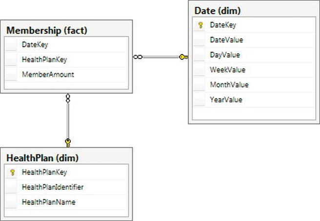
Figure 14-3. Snapshot fact dimensional model for our health care payer
In our healthcare example, daily member count is a perfect example of a snapshot fact. We begin by following a similar process to determine our dimensions and metrics. Our business process is listed below with dimensions in bold and metrics italicized:
An insurance company’s core business depends on its members. It is important to know how many members the company has over time, whether the number of members is increasing or decreasing, and which health plan is doing well over time.
We don’t have many dimensions attached to this fact based on the business process, but that’s OK because it supports our reporting questions. We have two main dimensions: the date and health plan. Our metrics are the number of members that we have. Note that we don’t have a member dimension because we are looking at an aggregation of the number of members over time, not individual members. It is important to provide this data on a time basis so that people can report historical information. Our final snapshot table can be created with the following script:
-- Create Membership snapshot fact table
CREATE TABLE fact.Membership (
DateKey INTEGER NOT NULL,
HealthPlanKey INTEGER NOT NULL,
MemberAmount INTEGER NOT NULL
)
GO
In addition, we need to add the foreign keys to link the fact table to our dimensions, using the following script:
-- Add foreign keys from Membership fact to dimensions
ALTER TABLE fact.Membership WITH CHECK
ADD CONSTRAINT FK_Membership_Date
FOREIGN KEY(DateKey) REFERENCES dim.Date (DateKey)
GO
ALTER TABLE fact.Membership WITH CHECK
ADD CONSTRAINT FK_Membership_HealthPlan
FOREIGN KEY(HealthPlanKey) REFERENCES dim.HealthPlan (HealthPlanKey)
GO
To load sample data into this table, use the following query:
-- Insert sample data into the Membership fact table
DECLARE @startdate DATE
DECLARE @enddate DATE
SET @startdate = '1/1/2011'
SET @enddate = '12/31/2011'
WHILE @startdate <= @enddate
BEGIN
INSERT INTO fact.Membership
SELECT CONVERT(CHAR(8), @startdate, 112) AS DateKey
,1 AS HPKey
,RAND() * 1000 AS MemberAmount
INSERT INTO fact.Membership
SELECT CONVERT(CHAR(8), @startdate, 112) AS DateKey
,2 AS HPKey
,RAND() * 1000 AS MemberAmount
INSERT INTO fact.Membership
SELECT CONVERT(CHAR(8), @startdate, 112) AS DateKey
,3 AS HPKey
,RAND() * 1000 AS MemberAmount
SET @startdate = DATEADD(dd, 1, @startdate)
END
GO
This type of fact table can get very large, because it contains data for every combination of keys. Although, in this case, the key combination is just day and health plan, imaging adding a few more dimensions, and see how quickly that would grow. What we lose in storage, however, we gain in power. As an example, the following query quickly illustrates how many members plan 2 had over time. We can use this information to show a line chart or a dashboard that shows trends.
select dd.DateValue, fm.MemberAmount
from fact.Membership fm
left join dim.Date dd on fm.DateKey = dd.DateKey
left join dim.HealthPlan dp on fm.HealthPlanKey = dp.HealthPlanKey
where dd.DateValue IN ('2011-09-01', '2011-09-02', '2011-09-03')
and fm.HealthPlanKey = 2
GO
This snapshot fact table is based on a daily grain, but showing snapshots on only a monthly grain instead is also common. This coarser grain can help the storage issue but should only be an alternative if the business process looks at the metrics on the monthly basis.
Recall that, from my outty perspective, the whole point of storing data is to get the information out, and we can write a variety of queries to get that information. Let’s start with a combination of our dimensions and transaction fact from the previous section to provide some information to our users. Then, we’ll look at how indexes can improve our query performance.
Our first reporting request is to deliver the number of claims that have had a payment denied over a certain length of time. For this query, we will use the fact.ClaimPayment table joined to some dimension tables:
select count(fcp.ClaimID) as DeniedClaimCount
from fact.ClaimPayment fcp
inner join dim.AdjudicationType da on fcp.AdjudicationTypeKey=da.AdjudicationTypeKey
inner join dim.Date dd on fcp.DateKey=dd.DateKey
where da.AdjudicationType = 'DENIED'
and dd.MonthValue = 9
GO
This query highlights a few querying best practices. First of all, try not to filter by the surrogate key values. Using surrogate keys is tempting, because we know that the key for the DENIED adjudication type is always going to be 3. Doing so would also remove a join, because we could filter directly on the claim payment fact. However, this makes the query less readable in the future, not only to other report writers but also to us.
Additionally, this query shows the importance of creating descriptive column and table aliases. Creating column aliases that are descriptive will make it easier to understand the output of the query. Also, creating table aliases and using them to describe columns will reduce the possible confusion in the future if you add new columns or modify the query.
Because we were smart in creating our model, we can actually improve the performance of this query even further by using our DeniedCount column. Essentially, the work we need to do in the query was already done in the load process, so we end up with the following query:
select sum(fcp.DeniedCount) as DeniedClaimCount
from fact.ClaimPayment fcp
inner join dim.Date dd on fcp.DateKey=dd.DateKey
where dd.MonthValue = 9
GO
Our next reporting query is to assist the operations department in determining how much we are paying out based on automatic adjudication per provider, as the company is always trying to improve that metric. We can use the same fact but modify our dimensions to create the following query:
select dp.OrganizationName, sum(fcp.AutoPayoutAmount) as AutoPayoutAmount
from fact.ClaimPayment fcp
inner join dim.Provider dp on fcp.ProviderKey=dp.ProviderKey
group by dp.OrganizationName
GO
Many of the principles from relational querying also apply to reporting queries. Among these are to make sure to use set-based logic where possible, avoid using select *, and restrict the query results whenever possible. If we take the previous query, we can improve it by adding a filter and focusing on the business need. Because the operations group wants to improve their automatic adjudication rate, it is looking at the value over time. Taking those two factors into account, our new query can be used to create a line chart of the automatic adjudication rate over time:
select dp.OrganizationName,
dd.MonthValue,
sum(fcp.AutoPayoutAmount)/sum(ClaimAmount)*100 as AutoRatio
from fact.ClaimPayment fcp
inner join dim.Provider dp on fcp.ProviderKey=dp.ProviderKey
inner join dim.Date dd on fcp.DateKey=dd.DateKey
where dd.DateValue between '01/01/2011' and '12/31/2011'
group by dp.OrganizationName, dd.MonthValue
GO
A request that I often receive is “I want everything.” While I recommend digging into the business need to truly understand the reasoning behind the request, sometimes “everything” is exactly what the situation calls for. If so, we could provide a query similar to this:
select dd.DateValue, dm.InsuranceNumber, dat.AdjudicationType,
dp.OrganizationName, ddiag.DiagnosisCode, dhcpc.ProcedureCode,
SUM(fcp.ClaimAmount) as ClaimAmount,
SUM(fcp.AutoPayoutAmount) as AutoPaymountAmount,
SUM(fcp.ManualPayoutAmount) as ManualPayoutAmount,
SUM(fcp.AutoAdjudicatedCount) as AutoAdjudicatedCount,
SUM(fcp.ManualAdjudicatedCount) as ManualAdjudicatedCount,
SUM(fcp.DeniedCount) as DeniedCount
from fact.ClaimPayment fcp
inner join dim.Date dd on fcp.DateKey=dd.DateKey
inner join dim.Member dm on fcp.MemberKey=dm.MemberKey
inner join dim.AdjudicationType dat on fcp.AdjudicationTypeKey=dat.AdjudicationTypeKey
inner join dim.Provider dp on fcp.ProviderKey=dp.ProviderKey
inner join dim.Diagnosis ddiag on fcp.DiagnosisKey=ddiag.DiagnosisKey
inner join dim.HCPCSProcedure dhcpc on fcp.ProcedureKey=dhcpc.ProcedureKey
group by dd.DateValue, dm.InsuranceNumber, dat.AdjudicationType,
dp.OrganizationName, ddiag.DiagnosisCode, dhcpc.ProcedureCode
GO
The result of this query provides a great base for a drill-through report, where an end user can see a high-level summary of information and drill into the details. Additional fields from each dimension can be included without affecting the grain of the query at this time.
Notice that, in each of the preceding queries, we start with the fact table and then add the appropriate dimensions. Using this approach focuses on the metrics and uses the entities as descriptors. If you every find that you are querying a dimension directly, revisit the business process, and see if you can create a new fact to alleviate this concern.
Indexing is typically used to increase the query speed, so it’s a perfect fit for reporting. Let’s look at the following query based off of our healthcare model and work through some performance tuning through indexing to speed up the query:
SELECT ProcedureKey, SUM(ClaimAmount) As ClaimByProcedure
FROM fact.ClaimPayment
GROUP BY ProcedureKey
GO
With no index, this results in the following query plan:
|--Stream Aggregate(GROUP BY:([ReportDesign].[fact].[ClaimPayment].[ProcedureKey]) DEFINE:([Expr1004]=SUM([ReportDesign].[fact].[ClaimPayment].[ClaimAmount])))
|--Sort(ORDER BY:([ReportDesign].[fact].[ClaimPayment].[ProcedureKey] ASC))
|--Table Scan(OBJECT:([ReportDesign].[fact].[ClaimPayment]))
The table scan is a sign that this query may take longer than we would wish. Let’s start with a nonclustered index with our procedure key to see how that speeds up our performance. Create the index with this script:
CREATE NONCLUSTERED INDEX NonClusteredIndex ON fact.ClaimPayment
(
ProcedureKey ASC
)
GO
By running the same query, we will see the same plan, so we were not able to make any performance gains. Next, let’s try a new feature in SQL Server 2012 called columnstore indexes. Rather than store index data per row, they store data by column. They are typical indexes in that they don’t change the structure of the data, but they do make the table read-only in SQL Server 2012 because of the complexity of maintaining them. For each of the columns referenced in a columnstore index, all of the data is grouped and stored together. A table may have only a single columnstore index, but because of the way that index is structured, every column referenced is basically valuable independently, unlike existing row indexes. Create a columnstore index using the following script:
CREATE NONCLUSTERED COLUMNSTORE INDEX ColumnStoreIndex ON fact.ClaimPayment
(
DateKey,
MemberKey,
AdjudicationTypeKey,
ProviderKey,
DiagnosisKey,
ProcedureKey,
ClaimID,
ClaimAmount,
AutoPayoutAmount,
ManualPayoutAmount,
AutoAdjudicatedCount,
ManualAdjudicatedCount,
DeniedCount
)
GO
When you run the query again, you can see that the plan has changed quite drastically:
|--Stream Aggregate(GROUP BY:([ReportDesign].[fact].[ClaimPayment].[ProcedureKey]) DEFINE:([Expr1004]=SUM([ReportDesign].[fact].[ClaimPayment].[ClaimAmount])))
|--Sort(ORDER BY:([ReportDesign].[fact].[ClaimPayment].[ProcedureKey] ASC))
|--Index Scan(OBJECT:([ReportDesign].[fact].[ClaimPayment].[ColumnStoreIndex]))
The index scan operator (rather than the table scan operator from the original query) shows that this query is working with a columnstore index. I won’t cover columnstore indexes in any more detail, but for fact tables and some dimensions with large numbers of rows and low cardinality columns, you may be able to get order of magnitude improvements in performance by simply adding this one index. For more details, check SQL Server Books Online in the topic “columnstore indexes.”
Summary Modeling for Aggregation Reporting
If you are interested in analytical reporting, a dimensional model will probably best suit your needs. On the other hand, in some scenarios, a full dimensional model is not necessary. Creating an aggregation table or set of tables with the desired information will work perfectly for you in these cases. This section covers the reasons why you would want to use summary tables over dimensional modeling, the pros and cons of using a summary table, and finally, how to create a summary table.
Methodologies do not exist for summary modeling, as the development is so specific to your exact need. You can create summary tables to show values over specific time frames, rollups of different children companies versus the entire parent company, or even every requested value for a customer. We will cover an example of something I have used successfully in the past.
Summary modeling is best used when the slicing and dicing that we normally associate with data warehousing is not necessary. The information provided from the table usually feeds a limited set of reports but is tied very tightly to the information needed. Some of the benefits of summary modeling follow:
- Increased speed due to the preaggregated values
- Ease of maintenance and understandability due to fewer joins
Before jumping into this solution, you’ll want to consider some disadvantages as well:
- fixed data granularity limits the type of reports that can be created.
- Details of the data are not available for further analytical research.
- Historical tracking, such as what is provided with slowly changing dimensions, is not available.
Once you’ve decided that the benefits outweigh the disadvantages, you are ready to begin the process. You must go through the same steps as described in the “Requirements Gathering Process” section earlier in this chapter. You start this section once you reach step 4.
Let’s use the same business process as described earlier: When an insurance company receives a claim for a member, the claim goes through an adjudication process. The claim can either be automatically adjudicated, manually adjudicated, or denied. As an insurance company, we need to know whether we adjudicated the claim, how much the physician requested based on the member’s diagnosis, and how much we are willing to pay for that procedure.
In addition, we’ve been told that we want to display the number of claims over time for each adjudication type in a report. We could show this information using the prior model, but how would we do this in a summary model? We will walk through the steps now to produce the final model shown in Figure 14-4.
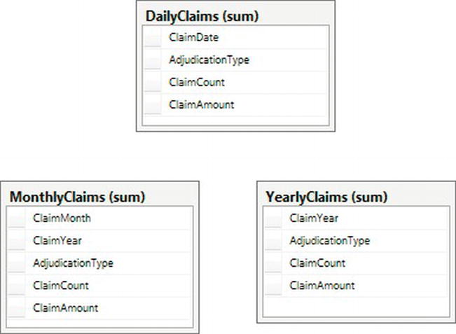
Figure 14-4. Summary model for health care claim data
Our first step is to determine the grain of our table. Using the business process description and report requirements, we see the grain includes: day, adjudication type, claim count, and claim amount. Unlike dimensional modeling, all codes and descriptive values are included in the aggregation table. Summary tables also do not use surrogate keys because there is no need to join tables together.
The code to create this table is shown here:
-- Create schema for summary tables
CREATE SCHEMA [sum]
GO
-- Create Daily Claims table
CREATE TABLE [sum].DailyClaims (
ClaimDate DATE NOT NULL,
AdjudicationType VARCHAR(6) NOT NULL,
ClaimCount INTEGER NOT NULL,
ClaimAmount DECIMAL(10,2) NOT NULL
)
GO
Note that the when you load the data, you will need to preaggregate the values to match your grain. For example, your claims system probably records more than one claim per day, but you want to see them all together! You can use SQL statements with SUM functions or Integration Services packages with the aggregate task, but either way, your insert should be the complete set of values. For a sample set of data, run the following query:
-- Add sample data for summary tables
DECLARE @i INT
SET @i = 0
WHILE @i < 1000
BEGIN
INSERT INTO sum.DailyClaims
(
ClaimDate, AdjudicationType, ClaimCount, ClaimAmount
)
SELECT
CONVERT(CHAR(8), DATEADD(dd, RAND() * -100, getdate()), 112),
CASE CEILING(3 * RAND())
WHEN 1 THEN 'AUTO'
WHEN 2 THEN 'MANUAL'
ELSE 'DENIED'
END,
1,
RAND() * 100000
SET @i = @i + 1
END
GO
The results that would be stored in the table could look similar to the following:
|
ClaimDate |
AdjudicationType |
ClaimCount |
ClaimAmount |
|
--------- |
---------------- |
---------- |
----------- |
|
2011-09-23 |
AUTO |
1 |
54103.93 |
|
2011-09-05 |
DENIED |
1 |
30192.30 |
|
2011-08-26 |
MANUAL |
1 |
9344.87 |
|
2011-09-06 |
DENIED |
1 |
29994.54 |
|
2011-06-25 |
AUTO |
1 |
52412.47 |
We’ve only completed part of our model though. What if report writers want to look at the adjudication types on a monthly, rather than daily, basis? Or even on a yearly basis? To satisfy these requirements, we will create two more tables:
-- Create Monthly Claims table
CREATE TABLE [sum].MonthlyClaims (
ClaimMonth INTEGER NOT NULL,
ClaimYear INTEGER NOT NULL,
AdjudicationType VARCHAR(6) NOT NULL,
ClaimCount INTEGER NOT NULL,
ClaimAmount DECIMAL(10,2) NOT NULL
)
GO
-- Create Yearly Claims table
CREATE TABLE [sum].YearlyClaims (
ClaimYear INTEGER NOT NULL,
AdjudicationType VARCHAR(6) NOT NULL,
ClaimCount INTEGER NOT NULL,
ClaimAmount DECIMAL(10,2) NOT NULL
)
GO
These tables can be loaded using the same method as before or by aggregating from the smaller-grained tables. Sample queries to load the month and year tables are shown here:
-- Add summarized data
insert into sum.MonthlyClaims
select MONTH(ClaimDate), YEAR(ClaimDate), AdjudicationType,
SUM(ClaimCount), SUM(ClaimAmount)
from sum.DailyClaims
group by MONTH(ClaimDate), YEAR(ClaimDate), AdjudicationType
GO
insert into sum.YearlyClaims
select YEAR(ClaimDate), AdjudicationType, SUM(ClaimCount), SUM(ClaimAmount)
from sum.DailyClaims
group by YEAR(ClaimDate), AdjudicationType
GO
When creating a model such as this one, it is tempting to create one supertable that includes all of the date grains: daily, monthly, and yearly. A table that does this would have another column named DateType where that row would describe each grain. While this option is valid, I prefer to make querying and maintenance easier and keep these as separate tables.
Because this is the section on reporting, we must talk about getting the information out of the tables we’ve designed! By design, the queries for summary tables are usually quite simple. We do have a few tricks up our sleeves to get the most out of our queries. Let’s look at some queries using the different grain table we created and then look at the best way to index the tables to get the best performance.
Let’s begin with the original request we received from the business: a way to see the number of claims over time for different adjudication types. Depending on what time the users are interested in, they will use one of the following very simple queries:
SELECT ClaimDate, AdjudicationType, ClaimCount, ClaimAmount
FROM sum.DailyClaims
GO
SELECT ClaimMonth, ClaimYear, AdjudicationType, ClaimCount, ClaimAmount
FROM sum.MonthlyClaims
GO
SELECT ClaimYear, AdjudicationType, ClaimCount, ClaimAmount
FROM sum.YearlyClaims
GO
This will return the exact information requested by the end user. It is important to still drill into what the end result of the report should look like for end users. For example, if they are only interested in seeing the last three months of data at the day level, we can write that query as such:
SELECT ClaimDate, AdjudicationType, ClaimCount, ClaimAmount
FROM sum.DailyClaims
WHERE ClaimDate BETWEEN DATEADD(mm, -3, getdate()) and getdate()
ORDER BY ClaimDate
GO
The previous query filters the data returned so that a smaller set of information needs to be consumed and the query will perform more quickly. This best practice is similar to others we’ve discussed, and a lot of the other query best practices that we’ve talked about previously in this book are also applicable on summary tables.
Our next query request deals with the output of the information. We need to see the claim amounts for each of the adjudication types split into separate columns to be able to easily create a line chart. In this scenario, we will use the MonthlyClaims table and the SQL Server PIVOT function. The new query is shown here:
SELECT ClaimMonth, ClaimYear, [AUTO], [MANUAL], [DENIED]
FROM
(SELECT ClaimMonth, ClaimYear, AdjudicationType, ClaimAmount
FROM sum.MonthlyClaims) AS Claims
PIVOT
(
SUM(ClaimAmount)
FOR AdjudicationType IN ([AUTO], [MANUAL], [DENIED])
) AS PivotedClaims
GO
This query works because we have a set list of values in the AdjudicationType field. Once we’ve successfully pivoted the information from rows to columns, the end user can use the results to create a report similar to the one shown in Figure 14-5.
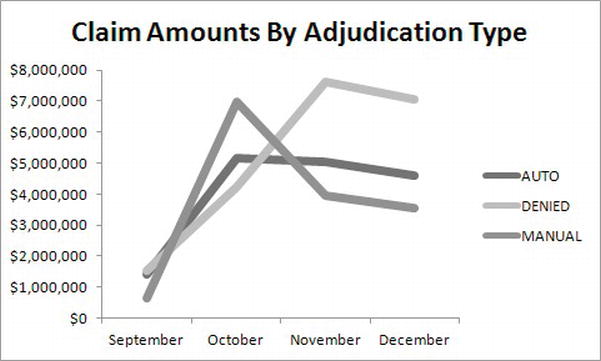
Figure 14-5. Sample claim amount report
Indexing is particularly important within summary tables, as users will often be searching for just one row. In particular, a covering index is a perfect fit. Let’s use a variation of our first simple query and build an index to support it. The query is
select SUM(ClaimCount) from sum.DailyClaims
where ClaimDate = '09/10/2011'
GO
With no index, we get a fairly poor plan with a table scan and stream aggregate, as shown here:
|--Compute Scalar(DEFINE:([Expr1004]=CASE WHEN [Expr1006]=(0) THEN NULL ELSE [Expr1007] END))
|--Stream Aggregate(DEFINE:([Expr1006]=Count(*), [Expr1007]=SUM([ReportDesign].[sum].[DailyClaims].[ClaimCount])))
|--Table Scan(OBJECT:([ReportDesign].[sum].[DailyClaims]), WHERE:([ReportDesign].[sum].[DailyClaims].[ClaimDate]=CONVERT_IMPLICIT(date,[@1],0)))
Luckily for us, we know that a covering index that includes the column in the where clause and the column being selected will greatly improve the performance. Create the index using the following script:
CREATE NONCLUSTERED INDEX NonClusteredIndex ON sum.DailyClaims
(
ClaimDate ASC,
ClaimCount
)
GO
We end up with the plan shown here, in which the index seek will definitely improve our performance:
|--Compute Scalar(DEFINE:([Expr1004]=CASE WHEN [Expr1006]=(0) THEN NULL ELSE [Expr1007] END))
|--Stream Aggregate(DEFINE:([Expr1006]=Count(*), [Expr1007]=SUM([ReportDesign].[sum].[DailyClaims].[ClaimCount])))
|--Index Seek(OBJECT:([ReportDesign].[sum].[DailyClaims].[NonClusteredIndex]), SEEK:([ReportDesign].[sum].[DailyClaims].[ClaimDate]=CONVERT_IMPLICIT(date,[@1],0)) ORDERED FORWARD)
Make sure to always create the index based on the intended usage of the table. Creating the correct indexing scheme will make both you and your end users happier!
Summary
This chapter took a sharp turn off the path of relational modeling to delve into the details of modeling for reporting. We covered why you would want to model a reporting database differently than a transactional system and the different ways we can model for reporting. I definitely did not cover every potential scenario you may face, but I hope I gave you a good introduction to get started with some initial reporting structures.
Dimensional modeling for analytical reporting and summary modeling for aggregate reporting serve different needs and requirements. Be sure to use the one most appropriate for your environment. Dimensional modeling, the better-known method, has several well-known methodologies, lead by Ralph Kimball and Bill Inmon. This chapter used ideas from both men, while explaining clearly and concisely some general dimensional modeling concepts. Summary modeling is a great first step toward reporting and can be very powerful. Be sure to understand the pros and cons of using this type of solution.
Finally, we looked at querying the different types of models. When designing for reporting, the end user and final queries should always be in the forefront. Without people who query, you have no need for a reporting database!