
Chapter 12
Tabular Models
What's in this chapter?
Introduction to PowerPivot
Importing data into PowerPivot
Explaining the PowerPivot window
Analyzing and enriching data
In Chapter 9 you learned about Microsoft Business Intelligence Semantic Model (BISM). You learned that it is made up of two components: multidimensional mode, which corresponds to the previous unified dimensional model (UDM), and tabular modeling, which is a more recent approach first implemented in the initial release of PowerPivot in SQL Server 2008 R2, with an add-in for Excel as the model development tool.
The Analysis Services team received a lot of positive feedback on PowerPivot. It considered different approaches for how to evolve it and make it available for corporate BI developers, as well as enable the underlying model for Power View for self-service business users performing highly interactive, visual analysis. SQL Server 2012 has two development tools for creating tabular models: an enhanced PowerPivot add-in for Excel and a new tabular development environment in Visual Studio for BI applications. This chapter focuses primarily on PowerPivot for Excel and covers these topics:
- Creating a tabular model using PowerPivot for Excel
- Enhancing a tabular model by integrating additional data
- Creating relationships between tables
- Analyzing data in a model through sorting and filtering
- Enriching a model by defining custom calculations
Introduction to PowerPivot
A key aspect of Microsoft's vision behind self-service business intelligence, as implemented in PowerPivot and Power View, is that your analytical data remains connected to its source. Also, it should be easy to update and refine your BI application and model to frequently evolving requirements. Furthermore, you can easily share data in a controlled way, and share visualizations and analyses built from the data.
PowerPivot is made up of two separate components that work together to accomplish this:
- PowerPivot for Excel is an Excel add-in that allows business analysts and Excel power users to create and edit tabular models within a tool they already know, Microsoft Office Excel.
- PowerPivot for SharePoint extends Microsoft Office SharePoint Server to include the ability to share and manage PowerPivot applications as well as tabular models created with PowerPivot for Excel.
PowerPivot applications are like Excel workbooks, but they include PowerPivot data and metadata embedded in the workbook. This enables PowerPivot workbooks to offer additional functionality over regular Excel workbooks. For example, PowerPivot workbooks can contain tables of hundreds of millions of rows of data; PowerPivot tables are not constrained by Excel tables, which can contain only 1 million rows of data (1,048,576 rows to be exact).
PowerPivot tables can be a source for Excel PivotTables and PivotCharts, as well as a source for Power View (which you'll read more about in Chapter 13) for reporting, analysis, and visualization. PowerPivot can represent relationships between tables and join tables just like a database. Figure 12.1 shows a PowerPivot workbook with multiple tables.

PowerPivot workbooks can be shared using Microsoft Office SharePoint Server. Workgroup members can then browse and interact with the workbook using the Excel client, a web browser (with Excel Services configured), or Power View. There is also PowerPivot Gallery, shown in Figure 12.2. This is a custom SharePoint document library type that previews workbook contents and provides an entry for creating a Power View analysis and visualization from a workbook, as discussed in Chapter 13.

PowerPivot workbooks can reference external data sources, for which you schedule automatic data refresh. Although manual data refresh can be accomplished directly within PowerPivot for Excel when the workbook is loaded, automatic data refresh uses PowerPivot for SharePoint and executes unattended on a specified schedule. As shown in Figure 12.3, you could configure an automatic data refresh for your workbook with the latest data every morning at 6.

To summarize, PowerPivot workbooks provide all the capabilities of Excel, plus additional modeling and analytical capabilities, to deliver self-service BI in conjunction with Excel and Reporting Services Power View.
PowerPivot for Excel
PowerPivot for Excel allows you to integrate data from various types of external data sources, link to existing data inside the workbook, add relationships between data, and enrich data with custom calculations. The data can then be used directly within Excel through features such as PivotTables and PivotCharts. You also can create highly interactive visualizations and analytical presentations with Power View.
PowerPivot for Excel includes the VertiPaq engine, a local version of the Analysis Services in-memory engine in VertiPaq mode that performs calculations and executes queries with high performance.
When you are working with PowerPivot for Excel, the data resides in memory. When you save the workbook, the data and metadata are stored inside the Excel workbook file.
PowerPivot for Excel is a free download on the web that can be found at http://powerpivot.com. It has the following prerequisites:
- .NET 3.5 SP1 — This component is automatically available on newer operating systems such as Windows 7. For older operating systems, you need to install .NET 3.5 SP1 before installing Office 2010. You can download .NET 3.5 SP1 from the Microsoft Download center at www.microsoft.com/download.
- Excel 2010 and Office Shared Features — PowerPivot for Excel requires Excel 2010; it won't install with earlier versions of Excel. An important feature of Excel 2010 is support for the 64-bit processor architecture. You have the option to choose a 64-bit or 32-bit installation. If you work with large quantities of data, you should use the 64-bit version. With the 32-bit version of the product, you are limited to a maximum of 2 GB of memory for Excel. PowerPivot for Excel also is limited to a maximum of 2 GB. The processor architecture of the Excel installation has to match the processor architecture of the PowerPivot add-in installation.
The installation of Office Shared Features is required because PowerPivot for Excel is a Visual Studio Tools for Office (VSTO) add-in and requires the VSTO runtime. The latter is installed when Office Shared Features are installed.
![]()
- Windows Vista / Windows Server 2008 Platform Update — If you are running Excel on the Vista or Windows Server 2008 operating system, PowerPivot for Excel requires the platform update described in KB 971644. You can download it at http://support.microsoft.com/kb/971644.
After you install these prerequisites and PowerPivot for Excel, start Microsoft Office Excel. A new command called PowerPivot Window appears on the Excel ribbon, as shown in Figure 12.4. This command is the entry point for PowerPivot for Excel. When you click it, the PowerPivot window opens, as shown in Figure 12.5.

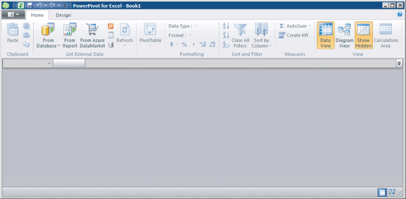
The PowerPivot Window provides commands to integrate data from various types of external data sources, linking to existing data inside the workbook, adding relationships between data, and enriching data with custom calculations. It provides a “window” into the PowerPivot data that is stored inside the workbook.
The following sections describe some of the key features of PowerPivot for Excel. You will work through a tutorial based on a sample relational database for SQL Server. It is called AdventureWorksDW_WroxSSRS2012 and is available on the Wrox download page for this book.
Setup and Installation
If you haven't installed Excel and PowerPivot for Excel, follow these steps:
Importing Data into PowerPivot
The PowerPivot window provides several ways to import data from various types of data sources, including the following:
- Relational data sources such as SQL Server, Oracle, and Teradata via OLE DB providers.
- Analysis Services or other PowerPivot workbooks.
- Existing reports rendered from Reporting Services.
- File-based data from Microsoft Access, Excel, and delimited text files.
- Data feeds such as RSS or Atom, SharePoint 2010 lists.
- Datasets from Azure DataMarket.
- Tables in an Excel worksheet. You can create a PowerPivot table from data on a worksheet in the Excel workbook. This links the PowerPivot table to the Excel table such that if the Excel table is updated, the PowerPivot table is automatically updated as well to match.
- Paste data from the Windows clipboard into a PowerPivot table if PowerPivot recognizes the clipboard data as tabular data.
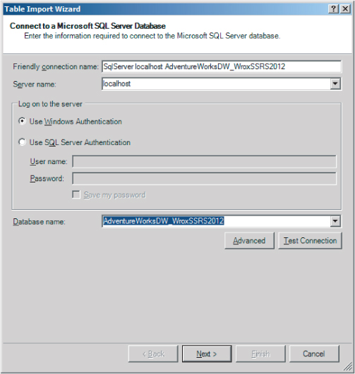
The following steps take you through an example of importing data from a SQL Server database that has the AdventureWorksDW_WroxSSRS2012 relational sample database deployed:

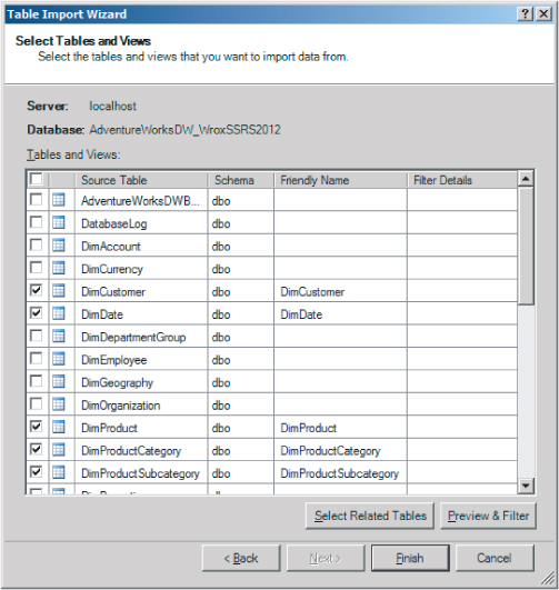
- DimCustomer
- DimDate
- DimProduct
- DimProductCategory
- DimProductSubcategory
- FactInternetSales
Editing the names in the Friendly Name column allows you to rename them immediately upon import. You can also rename them after the import is completed, directly in the PowerPivot window.
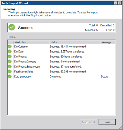
PowerPivot for Excel creates a data store utilizing the VertiPaq engine running in PowerPivot, and retrieves the data from the data source. You see the progress of these operations in the Importing page of the Table Import Wizard.
When importing tables directly, PowerPivot also tries to detect relationships between those tables in the data source system, to add them in the PowerPivot data store.
You can inspect the relationships created by clicking the Details link in the Message column of the import dialog, as shown in Figure 12.10.
If PowerPivot was unable to import relationships, the dialog provides more information on which relationships could not be successfully imported.
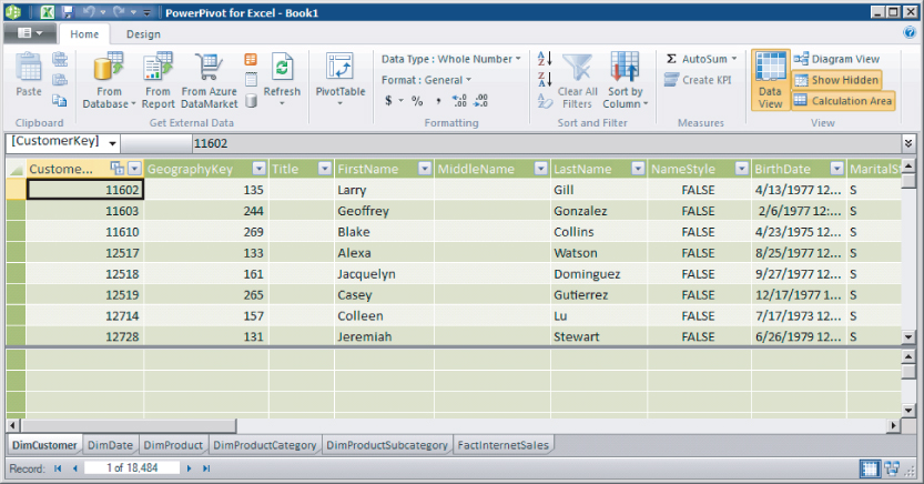
The PowerPivot window is now populated with all tables that have been imported. The default view of a model is Data View, where you can see a single table at a time and switch between them using tabs, such as Excel worksheet tabs, as shown in Figure 12.11. For each table, you see the columns of the table and data rows. You can select a cell value, and the Record indicator at the bottom of the window describes which record the cursor is currently positioned on. You can navigate rows within a table using the vertical scrollbar or the arrow buttons next to the Record indicator.
PowerPivot Window
With data imported, we can further enrich and refine the model. Before we do that, though, let's take a look at some of the features of the tabular designer. Figure 12.13 shows the PowerPivot tabular designer after our import is completed. Clicking the button to the left of the Home tab opens the File menu to save, and to toggle between Normal and Advanced mode. Advanced mode provides additional model options that are otherwise hidden in the PowerPivot window.
The Home Tab
The Home tab, shown in Figure 12.13, contains commands that apply to the model you are currently working on. The following is a brief description of its commands:
- Clipboard — This provides copy and paste actions, including appending rows to PowerPivot tables.
- Get External Data — This provides various import options: From Database, From Report, Azure DataMarket, Data Feed, Text, Other Sources. You saw these commands in action when you imported data into your model in the preceding section. You can also use them to import (additional) data into the model at any time.
- Refresh — This command refreshes your model with the current contents of the data sources. You can refresh from all data sources or just from a particular connection.
- PivotTable — This command creates a new PivotTable (or PivotChart) in the Excel workbook using your current tabular model as the source.
- Data Type — This command changes the data type of the selected column. The data type is autodetected on importing from the data source originally and can be changed afterwards.
- Format — These commands determine the textual formatting to apply when a particular column is used in a PivotTable or PivotChart in Excel, or when used in Power View.
- Sort and Filter — There offer various options that affect sorting and filtering of the table. The section “Analyzing and Enriching Data” explains them in more detail.
- AutoSum — AutoSum allows you to create a measure using common aggregation functions over the data in the currently selected column. AutoSum is covered later in this chapter in the “Measures” section.
- Create KPI — This command lets you create key performance indicator (KPI) visualizations for columns in the table.
- Data View / Diagram View — These commands switch between Data View (shown in Figure 12.11) and Diagram View (shown in Figure 12.12).
- Show Hidden — This command toggles whether hidden elements are shown in the designer.
- Calculation Area — This command toggles whether the calculation area below the rows of a table is shown in the tabular designer.
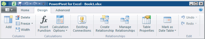
The Design Tab
The Design tab, shown in Figure 12.14, contains commands that affect individual model columns, define calculations, relationships, and table properties. The following is a brief description of its commands:
- Add — This command allows you to add a calculated column to the table. You'll learn about calculated columns later in this chapter.
- Delete — This command deletes the currently selected column or columns.
- Freeze — Freeze Column moves the currently selected columns to the far left of the table and freezes them. Freezing holds the columns in place regardless of the position of the horizontal scroll bar. You generally use this command when you want to see columns that are off the screen in relation to a particular column. The Unfreeze command removes the freeze action on frozen columns. They will scroll along with the rest of the columns when you move the horizontal scroll bar. Note that the Unfreeze command does not move the columns back to their original position.
- Width — This command adjusts the width of the selected table columns.
- Insert Function — This command inserts a new calculated column with a formula.
- Calculation Options — These commands control the calculation mode of the PowerPivot designer. In automatic calculation mode, calculations are updated automatically whenever the data changes. This can have performance implications for very large models with millions of rows or more. In automatic mode, the Calculate Now command is disabled.
You can use Calculation Options to change to manual calculation mode. In manual mode, the Calculate Now command is enabled, and calculations are updated only when you invoke the Calculate Now command.
- Existing Connections — This command brings up a dialog that lets you interact with all the data connections that are defined in the model. From that dialog you can import more data from an existing connection, edit an existing connection's properties, refresh the source data for a single connection, or delete a connection.
- Create Relationship and Manage Relationships — These commands allow you to work with relationships between tables. You'll learn about relationships in tabular mode later in this chapter.
- Table Properties — This command invokes the Edit Table Properties dialog. Here you can change the definition of the currently selected table, including the field import mapping from the table's data source.
- Mark as Date Table — The two commands under this menu item allow you to mark the currently selected table as a date table. This means that special date filtering functionality in Excel is enabled.
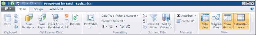
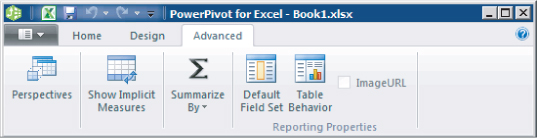
The Advanced Tab
The Advanced tab, shown in Figure 12.15, is visible only after PowerPivot switches from normal mode to advanced mode. This can be accomplished by clicking the top-left corner of the PowerPivot window to get to its File menu, which contains options for saving, asking questions, sending feedback, and switching between normal and advanced modes. The following is a brief description of the commands on the Advanced tab:
- Perspectives — This command brings up the perspectives dialog, which allows you to add or change the perspectives defined in the model. You can think of perspectives as multiple views (like database views) over the same underlying model tables.
- Show Implicit Measures — This toggles whether implicit measures are shown in the PowerPivot table designer. An implicit measure is generated automatically when a field is added to the Values area of the field list in an Excel PivotTable.
- Summarize By — This command determines the default aggregation function that reporting client tools, such as PowerPivot and Power View, apply when this column is added to a field list area. For example, you can change the default behavior of using a Sum aggregate to a DistinctCount aggregate. This command is enabled only for columns with numeric values.
- Table Behavior — This command enables you to change the default behavior of different visualization types and default grouping behavior in client tools, such as Power View, for the current table.
- Default Field Set — This command brings up the default field set dialog. Here you can specify the columns, measures, and field ordering that define the default field set when visualizing the selected table of your model in Power View. For example, you can define a set of default fields that should be picked when a business user initially selects an entire table to visualize.
- ImageURL — This command marks the selected column with metadata. Reporting clients such as Power View will treat the column's contents not as a string, but as a URL address of an image resource to download and visualize as an image in a report.
Analyzing and Enriching Data
This section describes some basic operations on tables using PowerPivot. Specifically, you'll learn about filtering and sorting, relationships, calculated columns, and measures.
Filtering and Sorting
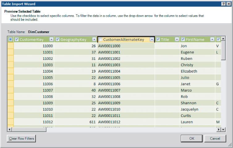
While importing data, you can apply filters and preview data. After importing data into PowerPivot, you can filter and sort data in a table in the PowerPivot window. For example, you can analyze sales data by following these steps:
Figure 12.16 shows the Filter drop-down in the PowerPivot window for a specific table column. Depending on the data type of the underlying field, custom filter options are available.
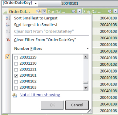
For example, fields that are whole numbers would show Number Filters with options for conditions such as greater than. For string columns, you would see Text Filters in the Filter drop-down.
With the sales data filtered to 99 rows for that particular date, you can view minimum and maximum sales by order on that date by sorting the SalesAmount column following these steps:

Sorting is performed over the filtered rows. It is very fast utilizing the VertiPaq engine in PowerPivot, even if the underlying dataset has millions of rows. By sorting, you can see that the maximum sales order on that day was $2,443.35, and the minimum sales order was $2.29.
Finally, on the Home tab, in the Sort and Filter section, select Clear All Filters to see all the data in the model again.
Relationships
An important aspect of the tabular model is relationships between tables. PowerPivot for Excel supports one-to-many relationships. This means that a column value in a specific table can have multiple instances of the value in another table's related column.
The table import wizard detects and understands the relationships that are present in the source data. It creates relationships in your model based on the relationships defined in the source data. In addition, the tabular designer provides ways to add relationships yourself.
If you are working in Data View, the designer indicates columns that participate in relationships with a glyph in the column header next to the column name. Hovering over the glyph provides details of the relationship. For example, hovering over the ProductKey column's glyph indicates “Related to [ProductKey] in table [DimProduct].” in a tooltip window.
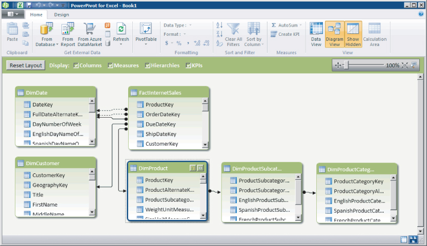
Diagram View provides a richer environment for working with relationships. You can see all the relationships in your model simultaneously in Diagram View. You can also work with them in a graphical way. For example, you can create new relationships by dragging and dropping from one column to the other. Follow these steps to add a new column to the model and manually create a relationship between it and an existing table:

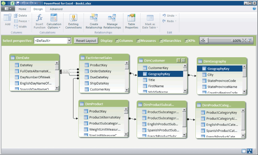
Alternatively, you can accomplish the same task using the Create Relationship command available on the Design tab. You can manage relationships by selecting Manage Relationships, which opens the dialog shown in Figure 12.20.

Relationships are a key part of the tabular model. The calculations that you create with DAX (Data Analysis Expressions) can use relationships to allow calculations that involve columns in different tables. Understanding when and how to create relationships in your model will help you realize your goals when analyzing your business data.
You can add DAX calculations to your model in two ways. The first, calculated columns, allows you to add expressions that define a new column in an existing table. You can refer to columns in the same table in your calculation, and the execution engine uses the value of the column in the current row as the calculation being evaluated. Another way to add calculations to your model is through what are called measures. Measures are calculations that are not done within the context of a table row. Rather, they are evaluated in the contents of the particular cell whose value they are being asked to provide.
Calculated columns and measures are explained in more detail in the following sections.
Calculated Columns
Similar to performing calculations on an Excel worksheet, PowerPivot allows you to create calculated columns and measures within the PowerPivot window using DAX functions. DAX functions are grouped into eight major categories:
- Date and Time
- Math and Trig
- Statistical
- Text
- Logical
- Filter
- Information
- Parent/Child
Calculated columns are useful when you need particular data values in your tables but those values are not in the data you have imported. It could be that you want to format data to display in a certain way in your client application. Or you may want to analyze a value that could be calculated from data values that are in the table. Or you may need a calculated column for some other purpose. The following steps show you how to add calculated columns to your model:

=RIGHT(" " & Format([MonthNumberOfYear],"#0"),2) & " - " & [EnglishMonthName]
You can verify the formula is correctly specified based on the values populating the calculated column (for example, “1 - January”).
=[SalesAmount] - [TotalProductCost]
You now know how to create calculated columns in PowerPivot. The columns you added are available in reporting client tools the same as any column that came from the source date. In this way, calculated columns allow you to customize the data for your model beyond the data you imported. This is a powerful capability of tabular mode.
Measures
Measures, like calculated columns, are defined by a DAX expression. Unlike calculated columns, they cannot refer to a particular column as a value unless an aggregation function has been applied to the column name. The values for measures are calculated on-the-fly at the time they are evaluated in the context that the value is being asked for. This section shows you how to work with measures.
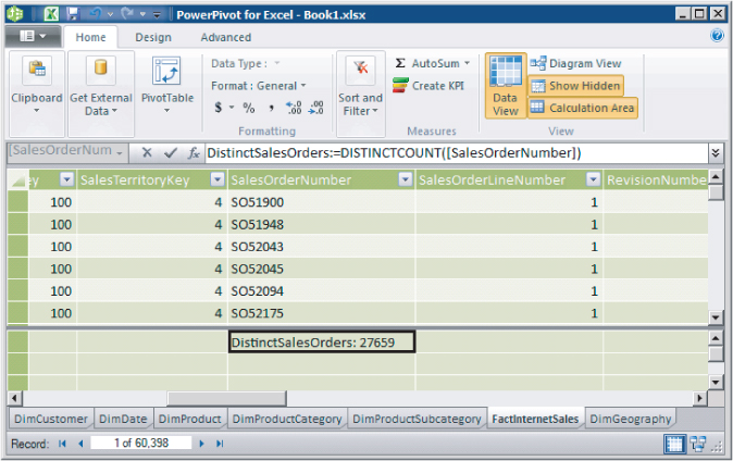
In the PowerPivot window, you work with measures in an area called the Calculation Area. (In the tabular designer in SQL Server Data Tools, the Calculation Area is called the Measure Grid.) The Calculation Area is the grid area below the splitter bar in the lower half of the Data View grid, as shown in Figure 12.22.

Follow these steps to create a measure in your model using the AutoSum feature:

You have now used the AutoSum function to create two measures. As you learn more about DAX, you will be able to create your own DAX measures to do more sophisticated analysis actions.
Browsing the Model
As you work with your tabular model, you may want to work with your tabular model in a client tool to verify it. Chapter 13 shows you how to accomplish this with Power View. You can also explore the model directly in Excel using a PivotTable or PivotChart by using the PivotTable menu on the Home tab, as shown in Figure 12.25.
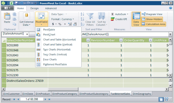
Figure 12.26 shows a PivotTable connected to the current model. Note that the measures you defined in the preceding section are available as values for analysis. The PivotTable shown in Figure 12.26 uses DimGeography.CountryRegionCode, FactInternetSales.DistinctSalesOrder, and FactInternetSales.InternetSalesAmount, which you created earlier.

Summary
This chapter gave you your first taste of working with PowerPivot for Excel, creating a tabular model. You learned about the commands available in the tabular designer and the two main model views, Data View and Diagram View. You walked through a simple scenario that showed the main components that make up a tabular model.
In the next chapter you'll learn about analyzing and visualizing your tabular models with Power View and creating exciting presentations in the process.