
Chapter 3. Processing
Processing was one of the first open source projects that was specifically designed for simplifying the practice of creating interactive graphical applications so that nonprogrammers could easily create artworks. Artists and designers developed Processing as an alternative to similar proprietary tools. It’s completely open source and free to download, use, and modify as you see fit. Casey Reas and Ben Fry started the project at MIT under the tutelage of John Maeda, but a group of developers maintain it by making frequent updates to the core application. The Processing project includes an integrated development environment (IDE) that can be used to develop applications, a programming language specifically designed to simplify programming for visual design, and tools to publish your applications to the web or to the desktop.
One of the reasons that we brought up the Java Virtual Machine (JVM) in the introduction is that Processing is a Java application; that is, it runs in the JVM. A Processing application that you as the artist create is also a Java application that requires the JVM to run. You can take two different approaches to running Processing applications. The first is running your Processing application on the Web, which means putting your application in a Hypertext Markup Language (HTML) page where a browser like Firefox, Internet Explorer, or Safari will encounter your application and start the JVM to run your application. The second is running your Processing application on the desktop, using the JVM that is installed on the user’s machine.
What can you do with Processing? Because Processing is built in Java and runs using Java, it can do almost anything Java will do, and although Java can’t quite do everything you’ll see in computational art and design, it certainly comes close. With it you can do everything from reading and writing data on the Internet; working with images, videos, and sound; drawing two- and three-dimensionally; creating artificial intelligence; simulating physics; and much more. If you can do it, there’s a very good chance you can do it using Processing.
In this chapter, we’ll cover the basics of getting started with Processing, including the following: downloading and installing the environment, writing some simple programs, using external libraries that let you extend what Processing is capable of, and running applications on the Internet and on the desktop.
Downloading and Installing Processing
The first step to installing Processing is to head to http://processing.org and look for the Download section. You’ll see four downloads, one for each major operating system (Windows, Mac OS X, and Linux) and one for Windows users who don’t want to install another instance of the JVM.
Processing includes an instance of the JVM, so you don’t need to worry about configuring your computer. In other words, everything Processing needs is right in the initial download. Download the appropriate archive for your operating system, and move the files in the archive to somewhere you normally store applications. On a Windows computer, this might be a location like C:Program FilesProcessing. On a Mac, it might be something like /Applications/Processing/. On a Linux machine, it might be somewhere like ~/Applications/.
Once you’ve downloaded and uncompressed the application, you’re done—you’ve installed Processing. Go ahead and start the application, and then type the following simple program in the window:
fill(0, 0, 255);
rect(0, 0, 100, 100);
print(" I'm working ");
Click the Run button (shown in the next section in Figure 3-1) to execute the program. This makes sure you have everything set up correctly. If this opens a new small window with a blue square in it and prints “I’m working” into the Console window, everything is good to go.
Exploring the Processing IDE
Before we talk about the IDE in detail, it’s important to understand the setup of the Processing environment. While the application is stored in your C:Program Files directory (for Windows users) or in your /Applications/ directory (for Mac or Linux users), the sketches that you create in Processing are usually stored in your home documents folder. This means that for a Windows user the default location for all your different sketches might be C:Documents And SettingsUserMy Documentsprocessing, for a Mac user it might be /Users/user/Documents/Processing/, and for a Linux user it might be home/user/processing/. You can always set this to a different location by opening Processing, opening the Preferences dialog and changing the “Sketchbook location” option to be wherever you’d like. The important thing is that you remember where it is.
Each Processing sketch you create and save will have its own folder. When you save a Processing sketch as image_fun, for example, a folder called image_fun will be created in the Processing project directory. If you’re planning on working with images, MP3 files, videos, or other external data, you’ll want to create a folder called data and store it in the project folder for the project that will use it. We’ll discuss this in greater detail in the section Importing Libraries. You can always view the folder for a particular sketch by pressing Ctrl+K (⌘-K on a Mac) when the sketch is open in the IDE.
As you can see in Figure 3-1, the Processing IDE has four main areas: the controls, the Code window, the Messages window, and the Console window.

The controls area is where all the buttons to run, save, stop, open, export, and create new applications appear. After you’ve entered any code in the Code window and you’re ready to see what it looks like when it runs, click the Run button, which opens a new window and runs your application in that window. To stop your application, either close the window or click the Stop button. The Export button creates a folder called applet within your project folder and saves all the necessary files there. You can find more information on this in the section Exporting Processing Applications later in this chapter.
The Code window is where you enter all the code for the application. It supports a few of the common text editor functions, like Ctrl-F (⌘-F on a Mac) for Find and Ctrl-Z (⌘-Z on a Mac) for Undo.
The Messages window is where any system messages that might appear will be shown. It isn’t widely used.
The Console window is where any trace statements or errors that occur while your application is running will be shown. Trace statements and printing messages to the consol will be discussed a little later on in this chapter.
The Basics of a Processing Application
A Processing application has two fundamental methods. These
methods are the instructions for your application at two core moments.
The first, setup(), is invoked when
the application first starts. The second, draw(), is invoked over and over again from
right after startup until the application closes. Let’s take a look at
the first of these and dissect what a method really is.
The setup() Method
Any instructions put in the setup() method run when the application
first starts. Conceptually, you can think of this as any kind of
preparation that you might be used to in daily life. Getting ready
to go for a run: stretch. Getting ready to fly overseas: make sure
you have a passport. Getting ready to cook dinner: check to see
everything you need is in the refrigerator. In terms of our
Processing application, the setup() method makes sure any information
you want to use in the rest of the application is prepared
properly.
Here’s an example:
void setup(){
    size(200, 200);
    frameRate(30);
    print(" all done setting up");
}
So, what’s going on in this code snippet? Well, first you have the return type of this method, and then you have its name. Taken together these are called the declaration of this method. If you don’t remember what a method declaration is, review Chapter 2. The rest of the code snippet is methods that have already been defined in the core Processing language. That is, you don’t need to redefine them, you simply need to pass the correct values to them.
The size() method
On the second line of the previous code snippet is the
size() method. It has two
parameters: how wide the
application is supposed to be and how tall it’s supposed to be,
both in pixels. This idea of measuring things in pixels is very
popular; you’ll see it in any graphics program, photo or video
editing program, and in the core code that runs all of these
programs. Get inches or centimeters out of your head; in this
world, everything is measured in pixels. This size()method makes the window that our
application is going to run in. Go ahead and write the previous
code in the Processing IDE, and click Run. Then change the size,
and click Run again. You’ll see that the size() method takes two
parameters:
void size(width, height)
Frequently when programmers talk about a method, they refer
to the signature of a method. This means what
parameters it takes and what values it returns. If this doesn’t
sound familiar, review Chapter 2,
specifically, the section on methods. In the setup() example, the size() method takes two integer (numbers
without any decimal values) values and returns void, that is, nothing.
The frameRate() method
The next method in the previous code snippet is the frameRate() method, which determines how
many frames per second your application is going to attempt to
display. Processing will never run faster than the frame rate you
set, but it might run more slowly if you have too many things
going at once or some parts of your code are inefficient. More
frames per second means your animations will run faster and
everything will happen more rapidly; however, it also can mean
that if you’re trying to do something too data intensive,
Processing will lag when trying keep up with the frame rate you
set. And how is this done? Well, the number you pass to the
frameRate() method is the
number of times per second that the draw() method is called.
The print() method
The print() method puts a
message from the application to the Console window in the
Processing IDE. You can print all sorts of things: messages,
numbers, the value of certain kinds of objects, and so forth.
These provide not only an easy way to get some feedback from your
program but also a simple way to do some debugging when things
aren’t working the way you’d like them to work. Expecting
something to have a value of 10? Print it to see what it really
is. All the print messages appear in the Console window at the
bottom of the Processing IDE, as shown in Figure 3-2.

The draw() Method
The draw() method is where
the drawing of the application happens, but it can be much more than
that. The draw() method is the
heartbeat of your application; any behavior defined in this method
will be called at the number of times per second specified as the
frame rate of your application.
This is a simple example of a draw() method:
void draw() {
println("hi");
}
Assuming that the frame rate of your application is 30 times a
second, the message "hi" will
print to the Console window of the Processing IDE 30 times a second.
That’s not very exciting, is it? But it demonstrates what the
draw() method is: the definition
of the behavior of any processing application at a regular interval
determined by the frame rate, after the application runs the
setup() method.
Now, let’s look at a slightly more interesting example and dissect it:
int x = 0;

void setup() {
    size(300, 300);
}

void draw() {
    // make x a little bit bigger
    x += 2;
    // draw a circle using x as the height and width of the circle
    ellipse(150, 150, x, x);
    // if x is too big, we can't see it in our window, so put it back
    // to 0 and start over
    if(x > 300) {
        x = 0;
    }
}
First things first—you’re making an int variable, x, to store a value:
int x = 0;
Since x isn’t inside a
method, it’s going to exist throughout the entire application. That
is, when you set it to 20 in the draw() method, then the next time the
draw() method is called the value
of x is still going to be 20.
This is important because it lets you gradually animate the value of
x.
To set up the application using the setup() method, simply set the size of the
window so that it’s big enough. Nothing much is too interesting
there, so you can skip right to the draw() method:
void draw() {Each time you call draw(),
you’re going to make this number bigger by 2. You could also write
x = x+2;, but the following is
simpler and does the same thing:
x += 2;
Now that you’ve made x a
little bit bigger, you can use it to draw a circle into the
window:
ellipse(150, 150, x, x);
Note
Look ahead in this chapter to the section The Basics of Drawing with Processing for more
information about the ellipse()
method.
If the value of x is too
high, the circle will be drawn too large for it to show up correctly
in your window (300 pixels); you’ll want to reset x to 0 so that the circles placed in the
window begin growing again in size:
    if(x > 300) {
        x = 0;
    }
}
In Figure 3-3,
you can see the animation about halfway through its cycle of
incrementing the x value and
drawing gradually larger and larger circles.

The draw() method is
important because the Processing application uses it to set up a lot
of the interaction with the application. For instance, the mousePressed() method and the mouseMove() methods that are discussed in
the section Capturing Simple User Interaction
will not work without a draw()
method being defined. You can imagine that the draw() method tells the application that
you want to listen to whatever happens with the application as each
frame is drawn. Even if nothing is between the brackets of the
draw() method, generally you
should always define a draw()
method.
The Basics of Drawing with Processing
Because Processing is a tool for artists, one of the most important tasks it helps you do easily is drawing. You’ll find much more information on drawing using vectors and bitmaps in Chapters 9 and 10, and you’ll find information about OpenGL, some of the basics of 3D, and how to create complex drawing systems in Chapter 13. For right now, you’ll learn how to draw simple shapes, draw lines, and create colors to fill in those shapes and lines.
The rect(), ellipse(), and line() Methods
Each of the three simplest drawing methods, rect(), ellipse(), and line(), lets you draw shapes in the
display window of your application. The rect() method draws a rectangle in the
display window and uses the following syntax:
rect(x, y, width, height)
Each of the values for the rect() method can be either int or float. The x and y
position variables passed to the rectangle determine the location of
the upper-left corner of the rectangle. This keeps in line with the
general rule in computer graphics of referring to the upper-left
corner as 0, 0 (to anyone with a math background this is a little
odd, since Cartesian coordinates have the y values flipped).
The ellipse() method is
quite similar to rect():
ellipse(x, y, width, height)
Each of the values passed to the ellipse() method can be int or float. If
you make the height and width of the ellipse the same, you get a
circle, of course, so you don’t need a circle() method.
Finally, the line() method
uses the following syntax:
line(x1, y1, x2, y2)
The x1 and y1 values define where the line is going
to start, and the x2 and y2 values define the end of the line.
Here’s a simple example incorporating each of the three
methods:
void setup() {
    size(300, 300);
}

void draw() {
    rect(100, 100, 50, 50);
    ellipse(200, 200, 40, 40);
    line(0, 0, 300, 300);
}
Notice in Figure 3-4 that because the line is drawn after the rectangle and ellipse, it’s on top of both of them. Each drawing command draws on top of what is already drawn in the display window.

Now, let’s take a brief interlude and learn about two ways to represent color.
RGB Versus Hexadecimal
There are two ways of representing colors in Processing in
particular and computing in general: RGB and hexadecimal. Both are
similar in that they revolve around the use of red, green, and blue
values. This is because the pixels in computer monitors are colored
using mixtures of these values to determine what color a pixel
should be. In RGB, you use three numbers between 0 and 255 and pass
them to the color() method. For
example, the following defines white:
int fullred = 255;
int fullgreen = 255;
int fullblue = 255;
color(fullred, fullgreen, fullblue);
Conversely, the following defines black:
int fullred = 0;
int fullgreen = 0;
int fullblue = 0;
color(fullred, fullgreen, fullblue);
All red and no green or blue is red, all green and blue and no red is yellow, and anytime all the numbers are the same the color is a gray (or white/black).
RGB is an easy way of thinking about color perhaps, but another way is commonly used on the Internet for HTML pages and has grown in popularity in other types of coding as well: hexadecimal numbers.
What’s a hexadecimal number? Well, a decimal number counts from 1 to 9 and then starts incrementing the number behind the 1. So, once you get to 9, you go to 10, and once you get to 19, you go to 20. This is the decimal system. The hexadecimal system is based on the number 16 and is very efficient for computers because computers like to process things in numbers that are cleanly divisible by 4 and 16, which 10 is not. A hexadecimal counting looks like this: 0, 1, 2, 3, 4, 5, 6, 7, 8, 9, A, B, C, D, E, F. So, that means that to write 13 in hexadecimal, you write D. To write 24, you write 18. To write 100, you write 64. The important concept is that to write 255, you write FF, which means representing numbers takes fewer characters to represent (“255” being three characters while “FF” is only two), which is part of where the efficiency comes from. Less characters means more efficient processing. Hexadecimal numbers for colors are written all together like this:
0xFF00FF
or:
#FF00FF
That actually says red = 255, green = 0, blue = 255, just in a
more efficient way. The 0x and
# prefixes tell the Processing
compiler you’re sending a hexadecimal number, not just mistyping a
number. You’ll need to use those if you want to use hexadecimal
numbers.
Here are some other colors:
000000= blackFFFFFF= white00FFFF= yellow
We’ll cover one final concept of hexadecimal numbers: the alpha value. The alpha value controls the transparency of a color and is indicated in hexadecimal by putting two more numbers at the beginning of the number to indicate, on a scale of 0–255 (which is really 0–FF), how transparent the color should be.
0x800000FF is an entirely
“blue” blue (that is, all blue and nothing else) that’s 50%
transparent. You can break it down into the following:
Alpha = 80 (that is, 50%)
Red = 00 (that is, 0%)
Green = 00 (that is, 0%)
Blue = FF (that is, 100%)
0xFFFF0000 is an entirely
“red” red, that is, 0% transparent or totally opaque with full red
values and no green or blue to mix with it, and 0x00FFFF00 is a magenta that is invisible.
This is why computer color is sometimes referred to as ARGB, which
stands for “alpha, red, green, blue.”
Now that you know the basics of colors, you can move on to using more interesting colors than white and black with shapes.
The fill() Method
The fill() method is named
as such because it determines what goes inside any shapes that have
empty space in them. Processing considers two-dimensional shapes
like rectangles and circles to be a group of points that have an
empty space that will be colored in by a fill color. Essentially,
imagine that setting the fill sets how any empty shapes will be
filled in. Without a fill, Processing won’t
know what color you want your shapes to be filled in with. The
fill() method lets you define the
color that will be used to fill in those shapes.
Before you really dive into the fill() method, it’s important to remember
that methods can be overloaded; that is, they
can have multiple signatures. If this doesn’t seem familiar to you
or you’d like a refresher on this, review Chapter 2.
The fill() method has many
different ways of letting you set the color that will be used to
fill shapes:
fill(int gray)This is an
intbetween 0 (black) and 255 (white).fill(int gray, int alpha)This is an
intbetween 0 (black) and 255 (white) and a second number for the alpha of the fill between 0 (transparent) and 255 (fully opaque).fill(int value1, int value2, int value3)Each of these values is a number between 0 and 255 for each of the following colors: red, green, and blue. For instance,
fill(255, 0, 0)is bright red,fill(255, 255, 255)is white,fill(255, 255, 0)is yellow, andfill(0, 0, 0)is black.fill (int value1, int value2, int value3, int alpha)This is the same as the previous example, but the additional
alphaparameter lets you set how transparent the fill will be.fill(color color)The
fill()method can also be passed a variable of typecolor, as shown here:void draw(){ color c = color(200, 0, 0); fill(c); rect(0, 0, 100, 100); }fill(color color, int alpha)When passing a variable of type
color, you can specify analphavalue:color c = color(200, 0, 0); fill(c, 150);fill(int hex)This is a fill using a hexadecimal value for the color, which can be represented by using the
0xprefix or the#prefix in the hexadecimal code. However, Processing expects that if you use0x, you’ll provide an alpha value in the hexadecimal code. This means if you don’t want to pass a separatealphavalue, use the0xprefix. If you do want to pass a separate alpha value, use the#prefix.fill(int hex, int alpha)This method uses a hexadecimal number but should be used with the
#symbol in front of the number, which can be a six-digit number only. The alpha value can be anywhere from 0 to 255.
The fill() method sets the
color that Processing will use to draw all shapes in the application
until it’s changed. For example, if you set the fill to blue like
so:
fill(0, 0, 255);
and then draw four rectangles, they will be filled with a blue color.
The background() Method
To set the color of the background window that your
application is running in, use the background() method. The background() method uses the same
overloaded methods as the fill()
method, with the method name changed to background(), of course. The background() method also completely covers
up everything that was drawn in the canvas of your application. When
you want to erase everything that has been drawn, you call the
background() method. This is
really helpful in animation because it lets you easily draw
something again and again while changing its position or size
without having all the previous artifacts hanging around.
The line() Method
You can use the line()
method in two ways. The first is for any two-dimensional
lines:
line(x1, y1, x2, y2)
The second is for any three-dimensional lines:
line(x1, y1, z1, x2, y2, z2)
Now, of course, a three-dimensional line will simply appear
like a two-dimensional line until you begin moving objects around in
three-dimensional space; we’ll cover that in Chapter 13. You need to take smaller steps
first. The line() method simply
draws a line from the point described in the first two (or three
parameters) to the point. You can set the color of the line using
the stroke() method and thickness
of the line using the strokeWeight() method.
The stroke() and strokeWeight() Methods
The stroke() method uses
the same parameters as the fill()
method, letting you set the color of the line either by using up to
four values from 0 to 255 or by using hexadecimal numbers. The
strokeWeight() method simply sets
the width of the lines in pixels. Let’s take a look:
void draw(){
    stroke(0xFFCCFF00); // here we set the color to yellow
    strokeWeight(5); // set the stroke weight to 5
    // draw the lines
    line(0, 100, 600, 400);
    line(600, 400, 300, 0);
    line(300, 0, 0, 100);
}
This draws a rectangular shape with yellow lines, 5 pixels thick.
The curve() Method
The curve() method draws a
curved line and is similar to the line() method except it requires you to
specify anchors that the line will curve toward.
You can use the curve()
method in two dimensions:
curve(x1, y1, x2, y2, x3, y3, x4, y4);
or in three dimensions:
curve(x1, y1, z1, x2, y2, z2, x3, y3, z3, x4, y4, z4);
All the variables here can be either floating-point numbers or
integers. The x1, y1, and z1 variables are the coordinates for the
first anchor point, that is, the first point that the curve will be
bent toward. The x2, y2, and z2 variables are the coordinates for the
first point, that is, where the line begins, in either two- or
three-dimensional space. The x3,
y3, and z3 parameters are the coordinates for the
second point, that is, where the line ends, and the x4, y4,
and z4 parameters are the
coordinates for the second anchor, that is, the second point that
the curve will be bent toward:
void setup(){
    size(400, 400);
}

void draw(){
    background(255);
    fill(0);
    int xVal = mouseX*3-100;
    int yVal = mouseY*3-100;
    curve(xVal, yVal, 100, 100, 100, 300, xVal, yVal);
    curve(xVal, yVal, 100, 300, 300, 300, xVal, yVal);
    curve(xVal, yVal, 300, 300, 300, 100, xVal, yVal);
    curve(xVal, yVal, 300, 100, 100, 100, xVal, yVal);
}
When this code snippet runs, you’ll have something that looks like Figure 3-5.

The vertex() and curveVertex() Methods
What is a vertex? A vertex is a point
where two lines in a shape meet, for example, at the point of a
triangle or point of a star. In Processing, you can use any three or
more vertices to create a shape with or without a fill by calling
the beginShape() method, creating
the vertices, and then calling the endShape() method. The beginShape() and endShape() methods tell the Processing
environment you intend to define points that should be joined by
lines to create a shape. Three vertices create a triangle, four a
quadrilateral, and so on. The Processing environment will create a
shape from the vertices that you’ve selected, creating lines between
those vertices, and filling the space within those lines with the
fill color you’ve defined. The following example creates three
vertices: one at 0, 0, which is the upper-left corner of the window;
one at 400, 400, which is the lower-right corner of the window; and
one at the user’s mouse position. The snippet results in the shape
shown in Figure 3-6.
void setup() {
    size(400, 400);
}

void draw(){
    background(255);
    fill(0);
    beginShape();
    vertex(0, 0);
    vertex(400, 400);
    vertex(mouseX, mouseY);
    endShape();
}
Capturing Simple User Interaction
To begin at the beginning, you’ll see how Processing handles the
two most common modes of user interaction: the mouse and the keyboard.
To capture interactions with these two tools, what you really need to
know is when the mouse is moving, when the mouse button has been
pressed, when the user is dragging (that is, holding the mouse button
down and moving the mouse), whether a key has been pressed, and what
key has been pressed. All these methods and variables already exist in
the Processing application. All you need to do is invoke them, that
is, to tell the Processing environment that you want to do something
when the method is invoked or access the variable either when one of
the methods is invoked or in the draw() method of your application.
The mouseX and mouseY Variables
The mouseX and mouseY variables contain the position of
the mouse in x and y coordinates. This is done in pixels, so if the
mouse is in the furthest upper-left corner of the window, mouseX is 0 and mouseY is 0. If the mouse pointer is in
the lower-right corner of a window that is 300 × 300 pixels, then
mouseX is 300 and mouseY is 300. You can determine the
position of the mouse at any time by using these variables. In the
following code snippet, you can determine the position of the mouse
whenever the draw() method is
called:
PFont arial;

void setup() {
    // make the size of our window
    size(300, 300);
    // load the font from the system
    arial = createFont("Arial", 32);
    // set up font so our application is using the font whenever
    // we call the text method to write things into the window
    textFont(arial, 15);
}

void draw() {
    // this makes the background black, overwriting anything there
    // we're doing this because we want to make sure we don't end up
    // with every set of numbers on the screen at the same time.
    background(0);
    // here's where we really do the work, putting the mouse position
    // in the window at the location where the mouse is currently
    text(" position is "+mouseX+" "+mouseY, mouseX, mouseY);
}
As you can see from the code comments, this example shows a
little more than just using the mouse position; instead, it uses the
text() method to put the position
of the mouse on the screen in text at the position of the mouse
itself. You do this by using the text() method, which takes three
parameters:
void text(string message, xPosition, yPosition);
The first parameter is the message, and the second and third
parameters can be floats or ints and are for positioning the
location of the text. In the previous example, you put the text
where the user’s mouse is using the mouseX and mouseY variables.
The mousePressed() Method
Processing applications have a mousePressed() method that is called
whenever the user clicks the left mouse button. This
callback method is called whenever the
application has focus and the user presses the mouse button. As
mentioned in the previous section, without a draw() method in your application, the
mousePressed() method will not
work. Let’s look at a quick example that uses a few drawing concepts
and also shows you how to use the mousePressed() method:
int alphaValue = 0;

void setup() {
    size(350, 300);
    background(0xFFFFFFFF);
}

void draw() {
    background(0xFFFFFFFF);
    fill(255, 0, 0, alphaValue);
    rect(100, 100, 100, 100);
}

void mousePressed() {
    print(mouseX + "
");
    alphaValue = mouseX;
}
The mousePressed() method
here sets the alpha value of the
fill that will be used when drawing the rectangle to be the position
of the user’s mouse. The application will draw using the alphaValue variable that is set each time
the mouse is clicked.
The mouseReleased() and mouseDragged() Methods
The mouseReleased() method
notifies you when the user has released the mouse button. It
functions similarly to the mousePressed() method and lets you create
actions that you would like to have invoked when the mouse button is
released. The mouseDragged()
method works much the same way, but is generally (though certainly
not always) used to determine whether the user is dragging the mouse
by holding the button down and moving the mouse around. Many times
when looking at mouse-driven applications you’ll see the mouseDragged() method being used to set a
boolean variable that indicates whether the user is dragging. In the
following example, though, you’ll put some actual drawing logic in
the mouseDragged()
method:
int lastX = 0;
int lastY = 0;

void setup() {
     size(400, 400);
}

void draw() {
    lastX = mouseX;
    lastY = mouseY;
}

void mouseDragged() {
    line(lastX, lastY, mouseX, mouseY);
}
Now you have a simple drawing application. You simply store
the last position of the user’s mouse and then, when the mouse is
being dragged, draw a line from the last position to the current
position. Try running this code and then comment out the lines in
the draw() method that set the
lastX and lastY variables to see how the application
changes.
An, easier way to do this is to use the pmouseX and pmouseY variables. These represent the x
and y mouse positions in the previous frame of the application. To
use these variables, you would use the following code:
void mouseDragged() {
    line(pmouseX, pmouseY, mouseX, mouseY);
}
To extend this a little bit, you’ll next create a slightly more complex drawing application that allows someone to click a location and have the Processing application include that location in the shape. This code sample has three distinct pieces that you’ll examine one by one. The first you’ll look at is a class that is defined in this example.
First, you have the declaration of the name of the class,
Point, and the bracket that
indicates you’re about to define all the methods and types of that
class:
class Point{Next, you have the two values that are going to store the
x and y values of Point:
float x;
    float y;
Here is the constructor for this class:
Point(float _x, float _y){
    x = _x;
    y = _y;
}
The constructor takes two values, _x and _y, and sets the x and y
values of Point to the two values
passed into the constructor. What this Point class now lets you do is store the
location where someone has clicked.
Now that you’ve defined the Point class, you can create an array of
those Point objects. Since you
want to allow for shapes with six vertices, in order to store them,
you’ll need an array of Point
instances with six elements:
Point[] pts = new Point[6];
Now all that’s left to do is set the mousePressed() method so that it stores
the mouseX and mouseY positions using the Point class and then draws all those
Point instances into the window.
We’ll break down each step of the code because this is pretty
complex:
Point[] pts = new Point[6];
int count = 0;
void setup(){
    size(500, 500);
}
In the draw() method, the
background is drawn filled in, the fill for any drawing is set using
the fill() method, and a for loop is used to draw a vertex for each
of the points:
void draw(){
    background(255);
    fill(0);
    beginShape();
    for(int i = 0; i<pts.length; i++){
Just to avoid any errors that may come from the Point object not being instantiated, you
check to make sure that the Point
in the current position in the array isn’t null:
if(pts[i] != null) {If it isn’t null, you’ll
use it to create a vertex using
Point from the pts array:
vertex(pts[i].x, pts[i].y);
        }
    }
Now you’re done drawing the shape:
endShape();
}
When the user presses the mouse, you want to store their mouse
position for use in the pts
array. You do this by creating a new Point object, passing it the current
mouseX and mouseY positions, and storing that in the
pts array at the count position:
void mousePressed(){
    if(count > 5){
        count = 0;
    }
    Point newPoint = new Point(mouseX, mouseY);
    pts[count] = newPoint;
    count++;
}
Finally, you have the declaration for the Point class:
class Point{
    float x;
    float y;
    Point(float _x, float _y){
        x = _x;
        y = _y;
    }
}
So, what happens when you click in the window? Let’s change
the Point class constructor
slightly so you can see it better:
Point(float _x, float _y){
        println(" x is: "+_x+" and y is "+_y);
        x = _x;
        y = _y;
    }
Now, when you click in the Processing window, you’ll see the following printed out in the Console window (depending on where you click, of course):
x is: 262.0 and y is 51.0
x is: 234.0 and y is 193.0
x is: 362.0 and y is 274.0
x is: 125.0 and y is 340.0
x is: 17.0 and y is 155.0
So, why is this happening? Look at the mousePressed(d) method again:
void mousePressed(){
...
    Point newPoint = new Point(mouseX, mouseY);
    pts[count] = newPoint;
}
Every time the mousePressed
event is called, you create a new Point, calling the constructor of the
Point class and storing the
mouseX and mouseY positions in the Point. Once you’ve created the Point object, you store the point in the
pts array so that you can use it
for placing vertices in the draw() method.
So, in the previous example, you’ll use for loops, classes, and arrays, as well as
the vertex() method. The last
code sample was a difficult one that bears a little studying.
There’s a lot more information on classes in Chapter 5.
The keyPressed and key Variables
Many times you’ll want to know whether someone is pressing a
key on the keyboard. You can determine when a key is pressed and
which key it is in two ways. The first is to check the keyPressed variable in the draw() method:
void draw() {
    if(keyPressed) {
        print(" you pressed "+key);
    }
}
Notice how you can use the key variable to determine what key is
being pressed. Any keypress is automatically stored by your
Processing application in this built-in variable.
Processing also defines a keyPressed() method that you can use in
much the same way as the mousePressed() or mouseMoved() method:
void keyPressed(){
    print(" you're pressing a key
 that key is "+key);
}
Any code to handle key presses should go inside the keyPressed() method. For instance,
handling arrow key presses in a game, or the user pressing the
Return button after they’ve entered their name in a text
field.
Importing Libraries
One of the great aspects of using Processing is the wide and varied range of libraries that have been contributed to the project by users. Most processing libraries are contained within .jar files. JAR stands for Java archive and is a file format developed by Sun that is commonly used for storing multiple files together that can be accessed by a Java application. In Processing applications, the Java application that will be accessing the .jar files is the Processing environment. When you include a library in a Processing code file and run the application, the Processing environment loads the .jar file and grabs any required information from the .jar and includes it in the application it’s building.
Downloading Libraries
Many Processing libraries are available for download at www.processing.org/reference/libraries/index.html. The libraries here include libraries used for working with 3D libraries, libraries that communicate with Bluetooth-enabled devices, and simple gesture recognition libraries for recognizing the movements made by a user with a mouse or Wii remote controller.
For this example, you’ll download the ControlP5 library, install it to the Processing directory, and write a quick test to ensure that it works properly. First, locate the ControlP5 library on the Libraries page of the Processing site under the Reference heading. Clicking ControlP5 on the Libraries page brings you to the ControlP5 page at http://www.sojamo.de/libraries/controlP5/. Once you’ve downloaded the folder, unzipping the .zip file will create the controlP5 folder. Inside this is a library folder that contains all the .jar files that the Processing application will access.
Now that you’ve downloaded the library, the libraries folder of your Processing sketchbook. The Processing sketchbook is a folder on your computer where all of your applications and libraries are stored. To change the sketchbook location, you can open the Preferences window from the Processing application and set value in the “Sketchbook location” field. You’ll need to copy the contributed library’s folder into the “libraries” folder at this location. To go to the sketchbook, you hit Ctrl-K (⌘-K on Mac OS X). If this is the first library you’ve added, then you need to create the “libraries” folder. For instance, on my computer the Processing sketchbook is installed at /Users/base/processing, so I place the controlP5 folder at /Users/base/processing/libraries/. Your setup may vary depending on where you’ve installed Processing and your system type. Once the library is in the correct location, restart the Processing IDE, and type the following code in the IDE window:
import controlP5.*;
Then, run the application. If a message appears at the bottom of the IDE saying this:
You need to modify your classpath, sourcepath,
 bootclasspath, and/or extdirs setup. Jikes could not find package
 "controlP5" in the code folder or in any libraries.
then the ControlP5 library has not been created properly. Double check that the folder is in the correct location. If you don’t get this message, you’ve successfully set up ControlP5. We’ll talk about it in greater depth in Chapter 7. For now, we’ll talk about some of the more common libraries for Processing and what they do:
- Minim by Damien Di Fede
This uses the JavaSound API to provide an easy-to-use audio library. This is a simple API that provides a reasonable amount of flexibility for more advanced users but is highly recommended for beginners. It’s clear and well documented.
- OCD by Kristian Linn Damkjer
The Obsessive Camera Direction (OCD) library allows intuitive control and creation of Processing 3D camera views.
- surfaceLib by Andreas Köberle and Christian Riekoff
This offers an easy way to create different 3D surfaces. It contains a library of surfaces and a class to extend.
- Physics by Jeffrey Traer Bernstein
This is a nice and simple particle system physics engine that helps you get started using particles, springs, gravity, and drag.
- AI Libraries by Aaron Steed
These are a great set of libraries to assist with artificial programming tasks such as genetic algorithms and the AStar pathfinding algorithm. We’ll discuss this in greater detail in Chapter 18.
- bluetoothDesktop by Patrick Meister
This library lets you send and receive data via Bluetooth wireless networks.
- proMidi by Christian Riekoff
This library lets Processing send and receive MIDI information.
- oscP5 by Andreas Schlegel
This library is an OpenSound Control (OSC) implementation for Processing. OSC is a protocol for communication among computers, sound synthesizers, and other multimedia devices.
Almost all of these will be discussed in later chapters when demonstrating how to extend Processing to help you work with physical interactions, other programming languages like Arduino, and other devices like GPS devices and physical controls.
Loading Things into Processing
Now that we’ve covered some of the basics of drawing with processing and some of the basics of capturing user interaction, you’ll learn how the Processing environment loads data, images, and movies. Earlier, we mentioned the default setup of a Processing project, with the folder data stored in the same folder as the .pde file. The Processing application expects that anything that’s going to be loaded into the application will be in that folder. If you want to load a file named sample.jpg, you should place it in the data folder within the same folder as the .pde file you’re working with.
Loading and Displaying Images
First, you’ll learn how to load images. One class and two
methods encapsulate the most basic approach to loading and
displaying images: the PImage
class, the loadImage() method,
and the image() method.
The PImage class
Processing relies on a class called PImage to handle displaying and sizing
images in the Processing environment. When you create a PImage object, you’re setting up an
object that can have an image loaded into it and then can be
displayed in the Processing environment. To declare a PImage object, simply declare it
anywhere in the application, but preferably at the top of the
code, as shown here:
PImage img;
Once you’ve declared the PImage object, you can load an image
into it using the loadImage() method.
The loadImage() method
This method takes as a parameter the name of an image file
and loads that image file into a PImage object. The name of the file can
be either the name of a file in the filesystem (in other words, in
the data folder of your
Processing applications home folder) or the name of a file using a
URL. This means you can do something like this to load a JPEG file
from the Internet:
    PImage rocks;
    rocks = loadImage("http://thefactoryfactory.com/images/hello.jpg");
Or you can do the following to load an image from the data folder within your Processing applications folder:
    PImage rocks;
    rocks = loadImage("hello.jpg");
The loadImage() method
lets you load JPEG, PNG, GIF, and TGA images. Other formats, such
as TIF, BMP, or RAW files, can’t be displayed by Processing
without doing some serious tinkering.
Now that you’ve looked at implementing the class that helps
you display images and you’ve seen how to load images into the
application, let’s look at actually displaying those images using
the image() method.
The image() method
The image() method takes
three parameters:
image(PImage, xPosition, yPosition);
The first is the PImage
object that should be displayed. If the PImage has not been created with
loadImage(), then trying to put
it on the screen using the image() method will cause an error.
There are ways around this, but we’ll leave those to Chapter 10. For now, let’s say that until a
PImage object has had an image
loaded into it, don’t try to use it with the image() method. The next two parameters
are the x and y positions of the upper-left corner of the image.
This is where the image will be displayed. Here’s a simple
example:
PImage img;

void setup() {
    size(400, 400);
    img = loadImage("sample.jpg");
    image(img, 0, 0);
}
As soon as the setup()
method is called, the window is given a size, the sample.jpg file is loaded into the
PImage, and the PImage is placed in the window at the 0,
0 position (that is, in the upper-left corner of the window). You
can also size the PImage using
the image() method. Like so
many methods in Processing, the image() method is overloaded, letting you pass
optional width and height values that will size the
image:
image(img, x, y, width, height)
By default, the image is displayed in the Processing window
at its default height and width, but you can also set the height and width of the image. Be aware, though,
that the image may have a different aspect ratio and might look
stretched or squashed slightly if using a size that doesn’t match
the original aspect ratio.
Displaying Videos in the Processing Environment
The Processing environment contains a Movie class to display videos. This class
relies on the Apple QuickTime video libraries, so if your computer
doesn’t have the QuickTime
libraries installed on it, you’ll need to download and install them
for your operating system. Note that at this time, working with
video in Processing on Linux is a fairly difficult and involved
process. The GSVideo library is fairly new and has a somewhat
difficult setup procedure; however, it does appear quite workable
and allows Linux users to work with different video formats in
Processing. For the sake of brevity in this book, we’ll leave you to
explore it on your own, if you’re curious.
Using the Movie Class
The Movie class lets you
load QuickTime movies; load movie files with .mov file extensions; play, loop, and
pause movies; change the speed; and tint the video. Creating a
Movie object is somewhat similar
to creating an image using the PImage class, with one important
distinction: you need to first import all the libraries that contain
the information about the Movie
class and how it works. These are all stored in a separate location
that can be accessed by using the import statement, as shown here:
import processing.video.*;
Next, declare a Movie
variable:
Movie mov;
In the setup() method, you
need to instantiate, or create, a new instance
of that Movie class. You do this
by calling the constructor of the Movie class. The constructor of the
Movie class is another overloaded
method that has four signatures:
Movie(parent, filename)
Movie(parent, filename, fps)
Movie(parent, url)
Movie(parent, url, fps)
The parent parameter is the
Processing application that will use and display the Movie class. For a simpler application,
the parent is almost always the application itself, which you can
reference using the this
keyword:
Movie(this, http://sample.com/movie.mov");
This isn’t vital to understand, but all Processing
applications are instances of a Java class called PApplet. The PApplet class handles calling the setup() and draw() methods and handling the mouse
movement and key presses. Sometimes, if you’re referencing a
Processing application from a child object loaded into it, the
parent PApplet will be the
application that your child is loaded into. This is fairly advanced
stuff and not something you’ll likely be dealing with, but if you
come across the parent parameter, the this keyword in an application, or the
PApplet,
you’ll know that all these things refer to the main application
class.
The filename and url parameters work much the same as they
do in the loadImage() method.
When loading a local file stored on the machine that the Processing
application is running on, use the filename of the .mov file. When loading a file from a
site on the Internet, use a URL. Finally, as an optional parameter,
you can pass a frame rate that the movie should be played at, if the
frame rate of your movie and the frame rate of the Processing
application are different. In the setup() method of this application, using
the reference to the Processing application and the local filename,
you’ll instantiate the Movie
object:
void setup() {
    size(320, 240);
    mov = new Movie(this, "sample.mov");
    mov.play();
}
In this code snippet, take a look at the play() method. This is important because
it tells the Processing environment to start reading from the movie
file right away. Without calling this method, the Processing
application won’t read the frames from the movie to display them.
It’s important to call either the play() or loop() method whenever you want the
Processing environment to begin displaying your movie.
To read a movie, you need to define a movieEvent() method in the application.
Why? Well, as the QuickTime Player plays the movie, it streams its
video in pieces or frames (not too different from the frames of a
film movie) to the Processing application, which then displays them
in the window. The movieEvent()
method is the QuickTime Player notifying the Processing environment
that a frame is ready to be displayed in much the same way that the
mousePressed() method is the
machine notifying the Processing environment that the mouse has
moved. To get the information for the frame, you want to call the
read() method of the Movie class. This reads the information
for the frame into the Movie
class and prepares the frame for display in the Processing
environment:
void movieEvent(Movie m) {
    m.read();
}
To draw the current frame of the movie into the window, you
use the image() method again just
the same as you did for a PImage
that contained all the information for a picture:
void draw() {
image(mov, 0, 0);
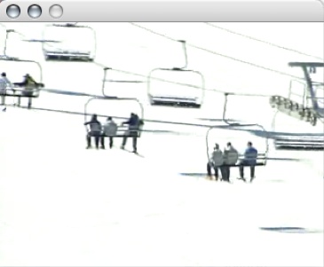
}This draws the current frame of the movie into the 0, 0, or upper-left, corner of the window. Figure 3-7 shows the results of the complete code listing:
import processing.video.*;
Movie mov;

void setup() {
    size(320, 240);
    mov = new Movie(this, "sample.mov");
    mov.play();
}

void movieEvent(Movie m) {
    m.read();
}

void draw() {
    image(mov, 0, 0);
}
Reading and Writing Files
The last thing to look at is reading in files. You can read in
a file in two ways, and the one you should use depends on the kind
of file you want to load. To load a picture, you would use the
loadImage() method; to load a
simple text file, you would use the loadStrings() method; and to load a file
that isn’t a text file, you would use the loadBytes() method. Since loading and
parsing binary data with the loadBytes() method are much more
involved, we’ll leave those topics for Chapter 12 and focus instead of
reading and writing simple text files.
The loadStrings() method
The LoadStrings() method
is useful for loading files that contain text and only text. This
means that loading more complex text documents like Microsoft Word
files isn’t going to work as smoothly as you’d like because they
contain lots of information other than just the text. Generally,
files with a .txt extension
or plain-text files without an extension are OK. This means that
files created in Notepad or in TextEdit will be loaded and
displayed without any problems. To load the file, you call the
loadStrings() method with either
the filename or the URL of the text that you want to
load:
loadStrings("list.txt");Now, that’s not quite enough, because you need to store the
data once you have loaded it. For that purpose, you’ll use an
array of String objects:
String lines[] = loadStrings("list.txt");This code makes the lines
array contain all the lines from the text file, each with its own
string in the array. To use these strings and display them, you’ll
create a for loop and draw each
string on the canvas using the text() method, as shown here:
void setup(){

    size(500, 400);

    PFont font;
    font = loadFont("Ziggurat-HTF-Black-32.vlw");
    textFont(font, 32);

    String[] lines = loadStrings("list.txt");
    print("there are " + lines.length + " lines in your file");
    for (int i=0; i < lines.length; i++) {
        text(lines[i], 20 + i*30, 50 + i*30);//put each line in a new place
    }
}
As a quick reminder, the text file that you load must be in the data folder of your Processing application or be downloaded from the Internet.
The saveStrings() method
Just as you can read strings from a text file with the
loadStrings() method, you can
write them out to a file just as easily. The process is somewhat
inverted. First, you make an array of strings:
String[] lines = new String[4];
lines[0] = "hello";
lines[1] = "out";
lines[2] = "there";
lines[3] = "!";
After creating an array, you can write the data back to a
file by passing its name to the saveStrings() method:
saveStrings("data/greeting.txt", lines);This creates and saves a file called greeting.txt with each element from the
lines array on a separate line
in the file.
Running and Debugging Applications
To run your application, simply click the Run button in the Processing IDE; you’ll see the output shown in Figure 3-8.

It couldn’t be easier, could it?
What happens when it doesn’t run? Look at the Message window in Figure 3-9.

Note the message, which is, in this case, very helpful:
The function printd(String) does not exist.
You see that the method you tried to call, printd(), doesn’t exist. The Processing
environment will also return deeper errors. For example, if you enter
the following line in a setup()
method:
frameRate(frames);
you may see this in the Console window:
No accessible field named "frames" was found in type "Temporary_85_2574".
This error indicates you’ve forgotten to define the variable frames. Change that line to this:
String frames = "foo";
frameRate(frames);
You’ll see the following in the Console window:
Perhaps you wanted the overloaded version "void frameRate(float $1):" instead?
This tells you the frameRate() method does not accept a string
as a parameter. Instead, it takes a float or an integer. Since the
Processing IDE always highlights the offending line, figuring out
which line is causing the problems tends to be quite easy. Some
errors, though, aren’t so easy to figure out. In these cases, checking
the Processing forums at http://processing.org/discourse/yabb_beta/YaBB.cgi is
usually your best bet. Thousands if not tens of thousands of
Processing users from all over the world ask and give advice on these
forums. If you’re having a problem, chances are someone has had it
before, asked there, and gotten an answer.
Exporting Processing Applications
Now, while running and debugging certainly helps when you want to see how the application is doing and check for errors in the code, it doesn’t much help when you’re trying to share it with a friend. To do that, you need to export the application.
The first step is to either select the Export Application option in the File menu or hit Ctrl-E (⌘+E on OS X). This will bring up a dialog, shown in Figure 3-10, asking you what operating systems you would like to create a dialog for.
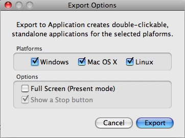
Once you click the Export button, you’ll be shown the location of your created executable files in your filesystem (Figure 3-11). There should be four folders, one for each operating system that you’ve created an application for and one for an applet that can run in a web browser. Each folder for the operating system version contains your application, compiled and ready to run on a desktop machine. The fourth folder contains the file necessary to place your application in a website where it can be viewed in a browser.
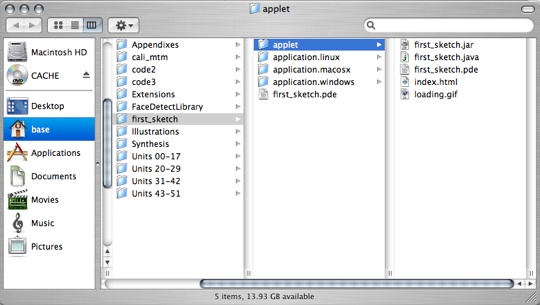
If you take a slightly closer look at what is generated by the export, you’ll see four distinct folders. The first folder is the applet folder. This folder contains all the files that you’ll need in order to put your Processing application on the Internet. You’ll see each file in the order that it appears in. This application is named first_sketch, so all the files will have that name:
- first_sketch.jar
This is the Java archive, or .jar file, that contains the Java runnable version of the sketch. When someone views the web page that contains your application, this file contains information about your application that will be used to run it.
- first_sketch.java
This is the Java code file that contains the code that the Java Virtual Machine will run to create your application.
- first_sketch.pde
This is your Processing code file.
- index.html
This is an HTML web page generated by the export that has the first_sketch.jar file embedded in it. When users open this page in a browser, if they do not have the correct Java runtime installed, a message directs them to the Sun site, where they can download it. This file is created, so that you can simply post the file to the Internet after you’ve created your application and have a ready-made page containing your Processing application.
- loading.gif
This .gif file is a simple image to show while the Java runtime is preparing to display your application.
So, in order to display your application online, simply place all the files in this folder in a publicly accessible location on a website.
The other three folders contain runnable executable versions of your processing application for each of the three major home operating systems: Windows, Mac OS X, and Linux. A Windows application for instance, has an .exe extension; an OS X application has an .app extension; and a Linux executable application doesn’t have any extension. Each of these three options lets you show your application outside the browser. If you have a friend who has a Windows computer that you want to send the Processing application to, you would simply compress the folder and all the files it contains into an archive and send it to that person. They could then unzip the file and run it by clicking the executable file. Each of these folders contains somewhat different files, but they all contain the .java file for their application and the Processing .pde file within their source folder. This is important to note because if you don’t want to share the source of your application, that is, the code that makes up your Processing application, remove this folder. If you want to share (remember that sharing is a good thing), then by all means leave it in and share your discoveries and ideas.
Conclusion
If you’re already thinking of exploring more about Processing, head to the Processing website at http://processing.org where you’ll find tutorials, exhaustive references, and many exhibitions of work made with Processing. Also, the excellent book, Processing: A Programming Handbook for Visual Designers and Artists (MIT Press), written by Casey Reas et al., provides a far more in-depth look at Processing than this chapter possibly could.
What next? Well, if you’re only interested in working with Processing, then skip ahead to Part II, where we explore different themes in computation and art and show you more examples of how to use Processing. If you’re interested in learning about more tools for creating art and design with, then continue with the next chapter. In Chapter 4, we discuss the open source hardware initiative that helps create physical interactions and integrates nicely with Processing.
Review
Processing is both an IDE and a programming language. Both are included in the download, which is available at processing.org/download.
Processing is based on the Java programming language, but is simplified to help artists and designers more easily prototype visual and interactive applications.
The Processing IDE has controls on the top toolbar to run an application; stop an application; and create, open, save, or export an application. All of these commands are also available in the File menu or as hotkeys.
Clicking the Run button compiles your code and starts running your application.
A Processing application has two primary methods: the setup() method, which is called when the
application starts up, and the draw() method, which is called at regular
intervals.
You set the number of times the draw() method is called per second using the
frameRate()
method.
The Processing drawing methods can be called within the draw() or setup() method, for example, with rect(), ellipse(), or line(). The method background() clears all drawing currently in
the display window.
When drawing any shape, the fill() method determines what color the fill
of the shape will be. If the noFill() method is called, then all shapes
will not use a fill until the fill() method is called again.
Processing defines mouseX and
mouseY variables to report the
position of the user’s mouse, as well as a key variable and a keyPressed() method to help you capture the
user’s keyboard input.
You can import libraries into Processing by downloading the
library files and placing them in the Processing libraries folder and restarting the
Processing IDE. Once the library has been loaded, you can use it in
your application with the import
statement to import all of its information, as shown here:
import ddf.minim.*; // just an example, using Minim
The PImage object and
loadImage() method allow you load
image files into your Processing application and display and
manipulate them.
The Movie class enables you
to load QuickTime movies into your application, display them, and
access their pixel data.
The saveStrings() and
loadStrings() methods let you load
data from text files, with a .txt
extension, and also to save data to those files.
The print() method is helpful
when debugging because it lets you trace the values of variables at
crucial points where their values are being changed.
The Processing IDE prints any error messages to the Console window at the bottom of the IDE. These messages can be helpful when trying to determine the cause of an error or bug. This Console window is also where any print messages are displayed.
You can export a Processing application as either a standalone executable, an .exe file for Windows, an .app file for Mac OS X, or you can export it for the Web as a Java applet.