
6
Trees and Graphs
Trees and graphs are common data structures, so both are fair game in a programming interview. Tree problems are more common, however, because they are simple enough to implement within the time constraints of an interview and enable an interviewer to test your understanding of recursion and runtime analysis. Graph problems are important but often more time-consuming to solve and code, so you won’t see them as frequently.
Unlike the previous chapter’s focus on implementations in C, this and subsequent chapters focus on implementations in more modern object-oriented languages.
TREES
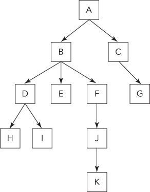
A tree is made up of nodes (data elements) with zero, one, or several references (or pointers) to other nodes. Each node has only one other node referencing it. The result is a data structure that looks like Figure 6-1.
As in a linked list, a node is represented by a structure or class, and trees can be implemented in any language that includes pointers or references. In object-oriented languages you usually define a class for the common parts of a node and one or more subclasses for the data held by a node. For example, the following are the C# classes you might use for a tree of integers:
public class Node {public Node[] children;}public class IntNode : Node {public int value;}
In this definition, children is an array that keeps track of all the nodes that this node references. For simplicity, these classes expose the children as public data members, but this isn’t good coding practice. A proper class definition would make them private and instead expose public methods to manipulate them. A somewhat more complete Java equivalent (with methods and constructors) to the preceding classes is:
public abstract class Node {private Node[] children;public Node( Node[] children ){this.children = children;}public int getNumChildren(){return children.length;}public Node getChild( int index ){return children[ index ];}}public class IntNode extends Node {private int value;public IntNode( Node[] children, int value ){super( children );this.value = value;}public int getValue(){return value;}}
This example still lacks error handling and methods to add or remove nodes from a tree. During an interview you may want to save time and keep things simple by using public data members, folding classes together, and sketching out the methods needed to manage the tree rather than fully implementing them. Ask interviewers how much detail they want and write your code accordingly. Any time you take shortcuts that violate good object-oriented design principles, be sure to mention the more correct design to the interviewer and be prepared to implement it that way if asked. This way you avoid getting bogged down in implementation details, but don’t give the impression that you’re a sloppy coder who can’t properly design classes.
Referring to the tree shown in Figure 6-1, you can see there is only one top-level node. From this node, you can follow links and reach every other node. This top-level node is called the root. The root is the only node from which you have a path to every other node. The root node is inherently the start of any tree. Therefore, people often say “tree” when talking about the root node of the tree.
Some additional tree-related terms to know are:
- Parent. A node that points to other nodes is the parent of those nodes. Every node except the root has one parent. In Figure 6-1, B is the parent of D, E, and F.
- Child. A node is the child of any node that points to it. In Figure 6-1, each of the nodes D, E, and F is a child of B.
- Descendant. All the nodes that can be reached by following a path of child nodes from a particular node are the descendants of that node. In Figure 6-1, D, E, F, H, I, J, and K are the descendants of B.
- Ancestor. An ancestor of a node is any other node for which the node is a descendant. For example, A, B, and D are the ancestors of I.
- Leaves. The leaves are nodes that do not have any children. G, H, I, and K are leaves.
Binary Trees
So far, we’ve used the most general definition of a tree. Most tree problems involve a special type of tree called a binary tree. In a binary tree, each node has no more than two children, referred to as left and right. Figure 6-2 shows an example of a binary tree.

The following is an implementation of a binary tree. For simplicity, everything is combined into a single class:
public class Node {private Node left;private Node right;private int value;public Node( Node left, Node right, int value ){this.left = left;this.right = right;this.value = value;}public Node getLeft() { return left; }public Node getRight() { return right; }public int getValue() { return value; }}
When an element has no left or right child, the corresponding reference is null.
Binary tree problems can often be solved more quickly than equivalent generic tree problems, but they are no less challenging. Because time is at a premium in an interview, most tree problems will be binary tree problems. If an interviewer says “tree,” it’s a good idea to clarify whether it refers to a generic tree or a binary tree.
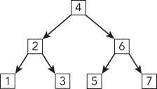
Binary Search Trees
Trees are often used to store sorted or ordered data. The most common way to store ordered data in a tree is to use a special tree called a binary search tree (BST). In a BST, the value held by a node’s left child is less than or equal to its own value, and the value held by a node’s right child is greater than or equal to its value. In effect, the data in a BST is sorted by value: all the descendants to the left of a node are less than or equal to the node, and all the descendants to the right of the node are greater than or equal to the node. Figure 6-3 shows an example of a BST.

BSTs are so common that many people mean a BST when they say “tree.” Again, ask for clarification before proceeding.
One advantage of a binary search tree is that the lookup operation (locating a particular node in the tree) is fast and simple. This is particularly useful for data storage. In outline form, the algorithm to perform a lookup in a BST is as follows:
Start at the root nodeLoop while current node is non-nullIf the current node's value is equal to the search valueReturn the current nodeIf the current node's value is less than the search valueMake the right node the current nodeIf the current node's value is greater than the search valueMake the left node the current nodeEnd loop
If you fall out of the loop, the node wasn’t in the tree.
Here’s an implementation of the search in C# or Java:
Node findNode( Node root, int value ){while ( root != null ){int curVal = root.getValue();if ( curVal == value ) break;if ( curVal < value ){root = root.getRight();} else { // curVal > valueroot = root.getLeft();}}return root;}
This lookup is fast because on each iteration you eliminate half the remaining nodes from your search by choosing to follow the left subtree or the right subtree. In the worst case, you will know whether the lookup was successful by the time there is only one node left to search. Therefore, the running time of the lookup is equal to the number of times that you can halve n nodes before you get to 1.
This number, x, is the same as the number of times you can double 1 before reaching n, and it can be expressed as 2x = n. You can find x using a logarithm.
For example, log2 8 = 3 because 23 = 8, so the running time of the lookup operation is O(log2(n)). Because logarithms with different bases differ only by a constant factor, it’s common to omit the base 2 and call this O(log(n)). log(n) is very fast. For an example, log2(1,000,000,000) ≈ 30.
One important caveat exists in saying that lookup is O(log(n)) in a BST: lookup is only O(log(n)) if you can guarantee that the number of nodes remaining to be searched will be halved or nearly halved on each iteration. Why? Because in the worst case, each node has only one child, in which case you end up with a linked list and lookup becomes an O(n) operation. This worst case may be encountered more commonly than you might expect, such as when a tree is created by adding data already in sorted order.
Binary search trees have other important properties. For example, you can obtain the smallest element by following all the left children and the largest element by following all the right children. The nodes can also be printed out, in order, in O(n) time. Given a node, you can even find the next highest node in O(log(n)) time.
Tree problems are often designed to test your ability to think recursively. Each node in a tree is the root of a subtree beginning at that node. This subtree property is conducive to recursion because recursion generally involves solving a problem in terms of similar subproblems and a base case. In tree recursion you start with a root, perform an action, and then move to the left or right subtree (or both, one after the other). This process continues until you reach a null reference, which is the end of a tree (and a good base case). For example, the preceding lookup operation can be reimplemented recursively as follows:
Node findNode( Node root, int value ){if ( root == null ) return null;int curVal = root.getValue();if ( curVal == value ) return root;if ( curVal < value ){return findNode( root.getRight(), value );} else { // curVal > valuereturn findNode( root.getLeft(), value );}}
Most problems with trees have this recursive form. A good way to start thinking about any problem involving a tree is to think recursively.
Heaps
Another common tree is a heap. Heaps are trees (usually binary trees) where (in a max-heap) each child node has a value less than or equal to the parent node’s value. (In a min-heap, each child is greater than or equal to its parent.) Consequently, the root node always has the largest value in the tree, which means that you can find the maximum value in constant time: simply return the root value. Insertion and deletion are still O(log(n)), but lookup becomes O(n). You cannot find the next higher node to a given node in O(log(n)) time or print out the nodes in sorted order in O(n) time as in a BST. Although conceptually heaps are trees, the underlying data implementation of a heap often differs from the trees in the preceding discussion.
You could model the patients waiting in a hospital emergency room with a heap. As patients enter, they are assigned a priority and put into the heap. A heart attack patient would get a higher priority than a patient with a stubbed toe. When a doctor becomes available, the doctor would want to examine the patient with the highest priority. The doctor can determine the patient with the highest priority by extracting the max value from the heap, which is a constant time operation.
Common Searches
It’s convenient when you have a tree with ordering properties such as a BST or a heap. Often you’re given a tree that isn’t a BST or a heap. For example, you may have a tree that is a representation of a family tree or a company organization chart. You must use different techniques to retrieve data from this kind of tree. One common class of problems involves searching for a particular node. When you search a tree without the benefit of ordering, the time to find a node is O(n), so this type of search is best avoided for large trees. You can use two common search algorithms to accomplish this task.
Breadth-First Search
One way to search a tree is to do a breadth-first search (BFS). In a BFS you start with the root, move left to right across the second level, then move left to right across the third level, and so forth. You continue the search until either you have examined all the nodes or you find the node you are searching for. A BFS uses additional memory because it is necessary to track the child nodes for all nodes on a given level while searching that level.
Depth-First Search
Another common way to search for a node is by using a depth-first search (DFS). A depth-first search follows one branch of the tree down as many levels as possible until the target node is found or the end is reached. When the search can’t go down any farther, it is continued at the nearest ancestor with unexplored children.
DFS has lower memory requirements than BFS because it is not necessary to store all the child pointers at each level. If you have additional information on the likely location of your target node, one or the other of these algorithms may be more efficient. For instance, if your node is likely to be in the upper levels of the tree, BFS is most efficient. If the target node is likely to be in the lower levels of the tree, DFS has the advantage that it doesn’t examine any single level last. (BFS always examines the lowest level last.)
For example, if you were searching a job hierarchy tree looking for an employee who started less than 3 months ago, you would suspect that lower-level employees are more likely to have started recently. In this case, if the assumption were true, a DFS would usually find the target node more quickly than a BFS.
Other types of searches exist, but these are the two most common that you will encounter in an interview.
Traversals
Another common type of tree problem is called a traversal. A traversal is just like a search, except that instead of stopping when you find a particular target node, you visit every node in the tree. Often this is used to perform some operation on each node in the tree. Many types of traversals exist, each of which visits and/or operates on nodes in a different order, but you’re most likely to be asked about the three most common types of depth-first traversals for binary trees:
- Preorder. Performs the operation first on the node itself, then on its left descendants, and finally on its right descendants. In other words, a node is always operated on before any of its descendants.
- Inorder. Performs the operation first on the node’s left descendants, then on the node itself, and finally on its right descendants. In other words, the left subtree is operated on first, then the node itself, and then the node’s right subtree.
- Postorder. Performs the operation first on the node’s left descendants, then on the node’s right descendants, and finally on the node itself. In other words, a node is always operated on after all its descendants.
Preorder and postorder traversals can also apply to nonbinary trees. Inorder traversal can apply to nonbinary trees as long as you have a way to classify whether a child is “less than” (on the left of) or “greater than” (on the right of) its parent node.
Recursion is usually the simplest way to implement a depth-first traversal.
GRAPHS
Graphs are more general and more complex than trees. Like trees, they consist of nodes with children—a tree is actually a special case of a graph. But unlike tree nodes, graph nodes (or vertices) can have multiple “parents,” possibly creating a loop (a cycle). In addition, the links between nodes, as well as the nodes themselves, may have values or weights. These links are called edges because they may contain more information than just a pointer. In a graph, edges can be one-way or two-way. A graph with one-way edges is called a directed graph. A graph with only two-way edges is called an undirected graph. Figure 6-4 shows a directed graph, and Figure 6-5 shows an undirected graph.
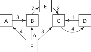
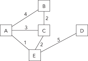
Graphs are commonly used to model real-world problems that are difficult to model with other data structures. For example, a directed graph could represent the aqueducts connecting cities because water flows only one way. You might use such a graph to help you find the fastest way to get water from city A to city D. An undirected graph can represent something such as a series of relays in signal transmission.
Several common ways exist to represent graph data structures. The best representation is often determined by the algorithm being implemented. One common representation has the data structure for each node include an adjacency list: a list of references to other nodes with which the node shares edges. This list is analogous to the child references of the tree node data structure, but the adjacency list is usually a dynamic data structure because the number of edges at each node can vary over a wide range. Another graph representation is an adjacency matrix, which is a square matrix with dimension equal to the number of nodes. The matrix element at position i,j represents the weight of the edge extending from node i to node j.
All the types of searches possible in trees have analogs in graphs. The graph equivalents are usually slightly more complex due to the possibility of cycles.
Graphs are often used in real-world programming, but they are less frequently encountered in interviews, in part because graph problems can be difficult to solve in the time allotted for an interview.
TREE AND GRAPH PROBLEMS
Most tree problems involve binary trees. You may occasionally encounter a graph problem, especially if the interviewer thinks you’re doing particularly well with easier problems.
Height of a Tree
Start by making sure you understand the definition provided in the problem for height of a tree (this is one of two common definitions). Then look at some simple trees to see if there’s a way to think recursively about the problem. Each node in the tree corresponds to another subtree rooted at that node. For the tree in Figure 6-2, the heights of each subtree are:
- A: height 4
- B: height 1
- C: height 3
- D: height 2
- E: height 2
- F: height 1
- G: height 1
- H: height 1
Your initial guess might be that the height of a node is the sum of the height of its children because height A = 4 = height B + height C, but a quick test shows that this assumption is incorrect because height C = 3, but the heights of D and E add up to 4, not 3.
Look at the two subtrees on either side of a node. If you remove one of the subtrees, does the height of the tree change? Yes, but only if you remove the taller subtree. This is the key insight you need: the height of a tree equals the height of its tallest subtree plus one. This is a recursive definition that is easy to translate to code:
public static int treeHeight( Node n ){if ( n == null ) return 0;return 1 + Math.max( treeHeight( n.getLeft() ),treeHeight( n.getRight() ) );}
What’s the running time for this function? The function is recursively called for each child of each node, so the function will be called once for each node in the tree. Since the operations on each node are constant time, the overall running time is O(n).
Preorder Traversal
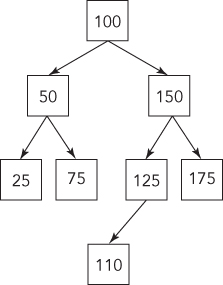
To design an algorithm for printing out the nodes in the correct order, you should examine what happens as you print out the nodes. Go to the left as far as possible, come up the tree, go one node to the right, and then go to the left as far as possible, come up the tree again, and so on. The key is to think in terms of subtrees.
The two largest subtrees are rooted at 50 and 150. All the nodes in the subtree rooted at 50 are printed out before any of the nodes in the subtree rooted at 150. In addition, the root node for each subtree is printed out before the rest of the subtree.
Generally, for any node in a preorder traversal, you would print the node itself, followed by the left subtree and then the right subtree. If you begin the printing process at the root node, you would have a recursive definition as follows:
- Print out the root (or the subtree’s root) value.
- Do a preorder traversal on the left subtree.
- Do a preorder traversal on the right subtree.
Assume you have a binary tree Node class with a printValue method. (Interviewers probably wouldn’t ask you to write out the definition for this class, but if they did, an appropriate definition would be the same as the Node class in the introduction to this chapter, with the addition of a printValue method.) The preceding pseudocode algorithm is easily coded using recursion:
void preorderTraversal( Node root ){if ( root == null ) return;root.printValue();preorderTraversal( root.getLeft() );preorderTraversal( root.getRight() );}
What’s the running time on this algorithm? Every node is examined once, so it’s O(n).
The inorder and postorder traversals are almost identical; all you vary is the order in which the node and subtrees are visited:
void inorderTraversal( Node root ){if ( root == null ) return;inorderTraversal( root.getLeft() );root.printValue();inorderTraversal( root.getRight() );}void postorderTraversal( Node root ){if ( root == null ) return;postorderTraversal( root.getLeft() );postorderTraversal( root.getRight() );root.printValue();}
Just as with the preorder traversal, these traversals examine each node once, so the running time is always O(n).
Preorder Traversal, No Recursion
Sometimes recursive algorithms can be replaced with iterative algorithms that accomplish the same task in a fundamentally different manner using different data structures. Consider the data structures you know and think about how they could be helpful. For example, you might try using a list, an array, or another binary tree.
Because recursion is so intrinsic to the definition of a preorder traversal, you may have trouble finding an entirely different iterative algorithm to use in place of the recursive algorithm. In such a case, the best course of action is to understand what is happening in the recursion and try to emulate the process iteratively.
Recursion implicitly uses a stack data structure by placing data on the call stack. That means there should be an equivalent solution that avoids recursion by explicitly using a stack.
Assume you have a stack class that can store nodes. Most modern languages include stack implementations in their standard libraries. If you don’t remember what the push and pop methods of a stack do, revisit the stack implementation problem in Chapter 5.
Now consider the recursive preorder algorithm, paying close attention to the data that is implicitly stored on the call stack so you can explicitly store the same data on a stack in your iterative implementation:
Print out the root (or subtree's root) value.Do a preorder traversal on the left subtree.Do a preorder traversal on the right subtree.
When you first enter the procedure, you print the root node’s value. Next, you recursively call the procedure to traverse the left subtree. When you make this recursive call, the calling procedure’s state is saved on the stack. When the recursive call returns, the calling procedure can pick up where it left off.
What’s happening here? Effectively, the recursive call to traverse the left subtree serves to implicitly store the address of the right subtree on the stack, so it can be traversed after the left subtree traversal is complete. Each time you print a node and move to its left child, the right child is first stored on an implicit stack. Whenever there is no child, you return from a recursive call, effectively popping a right child node off the implicit stack, so you can continue traversing.
To summarize, the algorithm prints the value of the current node, pushes the right child onto an implicit stack, and moves to the left child. The algorithm pops the stack to obtain a new current node when there are no more children (when it reaches a leaf). This continues until the entire tree has been traversed and the stack is empty.
Before implementing this algorithm, first remove any unnecessary special cases that would make the algorithm more difficult to implement. Instead of coding separate cases for the left and right children, why not push pointers to both nodes onto the stack? Then all that matters is the order in which the nodes are pushed onto the stack: you need to find an order that enables you to push both nodes onto the stack so that the left node is always popped before the right node.
Because a stack is a last-in-first-out data structure, push the right node onto the stack first, followed by the left node. Instead of examining the left child explicitly, simply pop the first node from the stack, print its value, and push both of its children onto the stack in the correct order. If you start the procedure by pushing the root node onto the stack and then pop, print, and push as described, you can emulate the recursive preorder traversal. To summarize:
Create the stackPush the root node on the stackWhile the stack is not emptyPop a nodePrint its valueIf right child exists, push the node's right childIf left child exists, push the node's left child
The code (with no error checking) for this algorithm is as follows:
void preorderTraversal( Node root ){Stack<Node> stack = new Stack<Node>();stack.push( root );while( !stack.empty() ){Node curr = stack.pop();curr.printValue();Node n = curr.getRight();if ( n != null ) stack.push( n );n = curr.getLeft();if ( n != null ) stack.push( n );}}
What’s the running time for this algorithm? Each node is examined only once and pushed on the stack only once. Therefore, this is still an O(n) algorithm. You don’t have the overhead of many recursive function calls in this implementation. On the other hand, the stack used in this implementation probably requires dynamic memory allocation and you may have overhead associated with calls to the stack methods, so it’s unclear whether the iterative implementation would be more or less efficient than the recursive solution. The point of the problem, however, is to demonstrate your understanding of trees and recursion.
Lowest Common Ancestor

Figure 6-7 suggests an intuitive algorithm: follow the lines up from each of the nodes until they converge. To implement this algorithm, make lists of all the ancestors of both nodes, and then search through these two lists to find the first node where they differ. The node immediately above this divergence is the lowest common ancestor. This is a good solution, but there is a more efficient one.
The first algorithm works for any type of tree but doesn’t use any of the special properties of a binary search tree. Try to use some of those special properties to help you find the lowest common ancestor more efficiently.
Consider the two special properties of binary search trees. The first property is that every node has zero, one, or two children. This fact doesn’t seem to help find a new algorithm.
The second property is that the left child’s value is less than or equal to the value of the current node, and the right child’s value is greater than or equal to the value of the current node. This property looks more promising.
Looking at the example tree, the lowest common ancestor to 4 and 14 (the node with value 8) is different from the other ancestors to 4 and 14 in an important way. All the other ancestors are either greater than both 4 and 14 or less than both 4 and 14. Only 8 is between 4 and 14. You can use this insight to design a better algorithm.
The root node is an ancestor to all nodes because there is a path from it to all other nodes. Therefore, you can start at the root node and follow a path through the common ancestors of both nodes. When your target values are both less than the current node, you go left. When they are both greater, you go right. The first node you encounter that is between your target values is the lowest common ancestor.
Based on this description, and referring to the values of the two nodes as value1 and value2, you can derive the following algorithm:
Examine the current nodeIf value1 and value2 are both less than the current node's valueExamine the left childIf value1 and value2 are both greater than the current node's valueExamine the right childOtherwiseThe current node is the lowest common ancestor
This solution may seem to suggest using recursion because it involves a tree and the algorithm repeatedly applies the same process to subtrees, but recursion is not necessary here. Recursion is most useful when each case has more than one subcase, such as when you need to examine both branches extending from each node. Here you are traveling a linear path down the tree. It’s easy to implement this kind of search iteratively:
Node findLowestCommonAncestor( Node root, int value1, int value2 ){while ( root != null ){int value = root.getValue();if ( value > value1 && value > value2 ){root = root.getLeft();} else if ( value < value1 && value < value2 ){root = root.getRight();} else {return root;}}return null; // only if empty tree}
What’s the running time of this algorithm? You travel down a path to the lowest common ancestor. Recall that traveling a path to any one node takes O(log(n)). Therefore, this is an O(log(n)) algorithm.
Binary Tree to Heap
To use an array sorting routine, as the problem requires, you must convert the tree you start with into an array. Because you both start and end with binary tree data structures, transforming into an array probably isn’t the most efficient way to accomplish the end goal. You might comment to your interviewer that if not for the requirement to use an array sorting routine, it would be more efficient to simply heapify the nodes of the starting tree: that is, reorder them such that they meet the criteria of a heap. You can heapify the tree in O(n) time, while just the array sort is at least O(n log(n)). But, as is often the case, this problem includes an arbitrary restriction to force you to demonstrate certain skills—here, it’s the ability to transform between tree and array data structures.
Your first task is to convert the tree into an array. You need to visit each node to insert its associated value into your array. You can accomplish this with a tree traversal. One wrinkle (assuming you’re working with static arrays) is that you have to allocate the array before you can put anything in it, but you don’t know how many values there are in the tree before you traverse it, so you don’t know how big to make the array. This is solved by traversing the tree twice: once to count the nodes and a second time to insert the values in the array. After the array has been filled, a simple call to the sorting routine yields a sorted array. The major challenge of this problem is to construct the heap from the sorted array.
The essential property of a heap is the relationship between the value of each node and the values of its children: less than or equal to the children for a min-heap and greater than or equal for a max-heap. The problem doesn’t specify a min-heap or max-heap; we’ll arbitrarily choose to construct a min-heap. Because each value in the sorted array is less than or equal to all the values that follow it, you need to construct a tree where the children of each node come from further down the array (closer to the end) than their parent.
If you made each node the parent of the node to the right of it in the array, you would satisfy the heap property, but your tree would be completely unbalanced. (It would effectively be a linked list.) You need a better way to select children for each node that leaves you with a balanced tree. If you don’t immediately see a way to do this, you might try working in reverse: Draw a balanced binary tree, and then put the nodes into a linear ordering (as in an array) such that parents always come before children. If you can reverse this process, you’ll have the procedure you’re looking for.
One simple way to linearly arrange the nodes while keeping parents ahead of children is by level: first the root (the first level of the tree), then both of its children (the second level), then all their children (the third level), and so on. This is the same order in which you would encounter the nodes in a breadth-first traversal. Think about how you can use the relationship you’ve established between this array and the balanced tree that it came from.
The key to constructing the balanced heap from the array is identifying the location of a node’s children relative to the node itself. If you arrange the nodes of a binary tree in an array by level, the root node (at index 0) has children at indexes 1 and 2. The node at index 1 has children at 3 and 4, and the node at 2 has children at 5 and 6. Expand this as far as you need to identify the pattern: it looks like each node’s children have indexes just past two times the parent’s index. Specifically, the children of the node at index i are located at 2i + 1 and 2i + 2. Verify that this works with an example you can draw out, and then consider whether this makes sense. In a complete binary tree, there are 2n nodes at each level of the tree, where n is the level. Therefore, each level has one more node than the sum of the nodes in all the preceding levels. So, it makes sense that the indexes of the children of the first node in a level would be 2i + 1 and 2i + 2. As you move further along the level, because there are two children for each parent, the index of the child must increase by two for every increase in the index of the parent, so the formula you’ve derived continues to make sense.
At this point, it’s worth stopping to consider where you are with this solution. You’ve ordered the elements in an array such that they satisfy the heap property. (Beyond just satisfying the heap property, they are fully ordered because you were required to perform a full sort: this additional degree of ordering is why this step was O(n log(n)) instead of just the O(n) that it would have been to merely satisfy the heap property.) You’ve also determined how to find the children of each node (and by extension, the parent of each node) within this array without needing the overhead of explicit references or pointers between them. Although a binary heap is conceptually a tree data structure, there’s no reason why you can’t represent it using an array. In fact, arrays using implicit links based on position are the most common underlying data representation used for binary heaps. They are more compact than explicit trees, and the operations used to maintain ordering within the heap involve exchanging the locations of parents and children, which is easily accomplished with an array representation.
Although the array representation of your heap is probably a more useful data structure, this problem explicitly requires that you unpack your array into a tree data structure. Now that you know how to calculate the position of the children of each node, that’s a fairly trivial process.
Because you’re both starting and ending with a binary tree data structure, you can take a shortcut in implementation by creating an array of node objects and sorting that, rather than extracting the integer from each node into an array. Then you can simply adjust the child references on these nodes instead of having to build the tree from scratch. A Java implementation looks like:
public static Node heapifyBinaryTree( Node root ){int size = traverse( root, 0, null ); // Count nodesNode[] nodeArray = new Node[size];traverse( root, 0, nodeArray ); // Load nodes into array// Sort array of nodes based on their values, using Comparator objectArrays.sort( nodeArray, new Comparator<Node>(){@Override public int compare( Node m, Node n ){int mv = m.getValue(), nv = n.getValue();return ( mv < nv ? -1 : ( mv == nv ? 0 : 1 ) );}});// Reassign children for each nodefor ( int i = 0; i < size; i++ ){int left = 2*i + 1;int right = left + 1;nodeArray[i].setLeft( left >= size ? null : nodeArray[left] );nodeArray[i].setRight( right >= size ? null : nodeArray[right] );}return nodeArray[0]; // Return new root node}public static int traverse( Node node, int count, Node[] arr ){if ( node == null )return count;if ( arr != null )arr[count] = node;count++;count = traverse( node.getLeft(), count, arr );count = traverse( node.getRight(), count, arr );return count;}
Unbalanced Binary Search Tree
This would be a trivial problem with a binary tree, but the requirement to maintain the ordering of a BST makes it more complex. If you start by thinking of a large BST and all the possible ways it could be arranged, it’s easy to get overwhelmed by the problem. Instead, it may be helpful to start by drawing a simple example of an unbalanced binary search tree, such as the one in Figure 6-8.

What are your options for rearranging this tree? Because there are too many nodes on the left and not enough on the right, you need to move some nodes from the left subtree of the root to the right subtree. For the tree to remain a BST, all of the nodes in the left subtree of the root must be less than or equal to the root, and all the nodes in the right subtree greater than or equal to the root. There’s only one node (7) that is greater than the root, so you won’t be able to move any nodes to the right subtree if 6 remains the root. Clearly, a different node will have to become the root in the rearranged BST.
In a balanced BST, half of the nodes are less than or equal to the root and half are greater or equal. This suggests that 4 would be a good choice for the new root. Try drawing a BST with the same set of nodes, but with 4 as the root, as seen in Figure 6-9. Much better! For this example, the tree ends up perfectly balanced. Now look at how you need to change the child links on the first tree to get to the second one.
The new root is 4 and 6 becomes its right child, so you need to set the right child of the new root to be the node that was formerly the root. You’ve changed the right child of the new root, so you need to reattach its original right child (5) to the tree. Based on the second diagram, it becomes the left child of the former root. Comparing the previous two figures, the left subtree of 4 and the right subtree of 6 remain unchanged, so these two modifications, illustrated in Figure 6-10, are all you need to do.

Will this approach work for larger, more complex trees, or is it limited to this simple example? You have two cases to consider: first where the “root” in this example is actually a child of a larger tree and second where the “leaves” in this example are actually parents and have additional nodes beneath them.
In the first case, the larger tree was a BST to begin with, so we won’t violate the BST properties of the larger tree by rearranging the nodes in a subtree—just remember to update the parent node with the new root of the subtree.
In the second case, consider the properties of the subtrees rooted at the two nodes that get new parents. We must make sure that the properties of a BST won’t be violated. The new root was the old root’s left child, so the new root and all of its original children are less than or equal to the old root. Therefore there’s no problem with one of the new root’s child subtrees becoming the left subtree of the old root. Conversely, the old root and its right subtree are all greater than or equal to the new root, so there’s no problem with these nodes being in the right subtree of the new root.
Because there’s no case in which the properties of a BST will be violated by the transformation you’ve devised, this algorithm can be applied to any BST. Moreover, it can be applied to any subtree within a BST. You can imagine that a badly unbalanced tree could be balanced by applying this procedure repeatedly; a tree unbalanced to the right could be improved by applying the procedure with the sides reversed.
At some point during this problem, you may recognize that the algorithm you’re deriving is a tree rotation (specifically, a right rotation). Tree rotations are the basic operations of many self-balancing trees, including AVL trees and red-black trees.
Right rotation can be implemented as:
public static Node rotateRight( Node oldRoot ){Node newRoot = oldRoot.getLeft();oldRoot.setLeft( newRoot.getRight() );newRoot.setRight( oldRoot );return newRoot;}
An equivalent implementation as a nonstatic method of the Node class is better object-oriented design:
public Node rotateRight() {Node newRoot = left;left = newRoot.right;newRoot.right = this;return newRoot;}
rotateRight performs a fixed number of operations regardless of the size of the tree, so its run time is O(1).
Six Degrees of Kevin Bacon
The data structure you need to devise seems to involve nodes (actors) and links (movies), but it’s a little more complicated than the tree structures you’ve been working with up to this point. For one thing, each node may be linked to an arbitrarily large number of other nodes. There’s no restriction on which nodes may have links to each other, so it’s expected that some sets of links will form cycles (circular connections). Finally, there’s no hierarchical relationship between the nodes on either side of a link. (At least in your data structure; how the politics play out in Hollywood is a different matter.) These requirements point toward using a very general data structure: an undirected graph.
Your graph needs a node for each actor. Representing movies is trickier: each movie has a cast of many actors. You might consider also creating nodes for each movie, but this makes the data structure considerably more complicated: there would be two classes of nodes, with edges allowed only between nodes of different classes. Because you only care about movies for their ability to link two actors, you can represent the movies with edges. An edge connects only two nodes, so each single movie will be represented by enough edges to connect all pairs of actor nodes in the cast. This has the disadvantage of substantially increasing the total number of edges in the graph and making it difficult to extract information about movies from the graph, but it simplifies the graph and the algorithms that operate on it.
One logical approach is to use an object to represent each node. Again, because you only care about movies for establishing links, if two actors have appeared in more than one movie together, you need to maintain only a single edge between them. Edges are often implemented using references (or pointers), which are inherently unidirectional: there’s generally no way for an object to determine what is referencing it. The simplest way to implement the undirected edges you need here is to have each node object reference the other. An implementation of the node class in Java might look like:
public class ActorGraphNode{private String name;private Set<ActorGraphNode> linkedActors;public ActorGraphNode( String name ){this.name = name;linkedActors = new HashSet<ActorGraphNode>();}public void linkCostar( ActorGraphNode costar ){linkedActors.add( costar );costar.linkedActors.add( this );}}
The use of a Set to hold the references to other nodes allows for an unlimited number of edges and prevents duplicates. The graph is constructed by creating an ActorGraphNode object for each actor and calling linkCostar for each pair of actors in each movie.
Using a graph constructed from these objects, the process to determine the Bacon number for any actor is reduced to finding the length of the shortest path between the given node and the “Kevin Bacon” node. Finding this path involves searching across the graph. Consider how you might do this.
Depth-first searches have simple recursive implementations—would that approach work here? In a depth-first search, you repeatedly follow the first edge of each node you encounter until you can go no further, then backtrack until you find a node with an untraversed second edge, follow that path as far as you can, and so on. One challenge you face immediately is that unlike in a tree, where every path eventually terminates in a leaf node, forming an obvious base case for recursion, in a graph there may be cycles, so you need to be careful to avoid endless recursion. (In this graph, where edges are implemented with pairs of references, each edge effectively forms a cycle between the two nodes it connects, so there are a large number of cycles.)
How can you avoid endlessly circling through cycles? If a node has already been visited, you shouldn’t visit it again. One way to keep track of whether a node has been visited is to change a variable on the node object to mark it as visited; another is to use a separate data structure to track all the nodes that have been visited. Then the recursive base case is a node with no adjacent (directly connected by an edge) unvisited nodes. This provides a means to search through all the (connected) nodes of the graph, but does it help solve the problem?
It’s not difficult to track the number of edges traversed from the starting node—this is just the recursion level. When you find the target node (the node for the actor whose Bacon number you’re determining), your current recursion level gives you the number of edges traversed along the path you traveled to this node. But you need the number of edges (links) along the shortest path, not just any path. Will this approach find the shortest path? Depth-first search goes as far into the network as possible before backtracking. This means that if you have a network where a node could be reached by either a longer path passing through the starting node’s first edge, or a shorter path passing through the second edge, you will encounter it by the longer path rather than the shorter. So in at least some cases this approach will fail to find the shortest path; in fact, if you try a few more examples, you’ll find that in most cases the path you traverse is not the shortest. You might consider trying to fix this by revisiting previously visited nodes if you encounter them by a shorter path, but this seems overly complicated. Put this idea on hold and see if you can come up with a better algorithm.
Ideally, you want a search algorithm that encounters each node along the shortest path from the starting node. If you extend your search outward from the starting node in all directions, extending each search path one edge at a time, then each time you encounter a node, it will be via the shortest path to that node. This is a description of a breadth-first search. You can prove that this search will always find nodes along the shortest path: when you encounter an unvisited node while you are searching at n edges from the start node, all the nodes that are n – 1 or fewer edges from the start have already been visited, so the shortest path to this node must involve n edges. (If you’re thinking that this seems simpler than what you remember for the algorithm for finding the shortest path between two nodes in a graph, you may be thinking of Dijkstra’s algorithm. Dijkstra’s algorithm, which is somewhat more complex, finds the shortest path when each edge is assigned a weight, or length, so the shortest path is not necessarily the path with the fewest edges. Breadth-first search is sufficient for finding the shortest path when the edges have no [or equal] weights, such as in this problem.)
You may remember how to implement a breadth-first search for a graph, but we’ll assume you don’t and work through the details of the implementation. Just as with the depth-first search, you have to make sure you don’t follow cycles endlessly. You can use the same strategy you developed for the depth-first search to address this problem.
Your search starts by visiting each of the nodes adjacent to the starting node. You need to visit all the unvisited nodes adjacent to each of these nodes as well, but not until after you visit all the nodes adjacent to the start node. You need some kind of data structure to keep track of unvisited nodes as you discover them so that you can come back to them when it is their turn. Each unvisited node that you discover should be visited, but only after you’ve already visited all the previously discovered unvisited nodes. A queue is a data structure that organizes tasks to be completed in the order that they’re discovered or added: you can add unvisited nodes to the end of the queue as you discover them and remove them from the front of the queue when you’re ready to visit them.
A recursive implementation is natural for a depth-first search where you want to immediately visit each unvisited node as soon as you discover it and then return to where you left off, but an iterative approach is simpler here because the nodes you need to visit are queued. Prepare the queue by adding the start node. On each iterative cycle, remove a node from the front of the queue, and add each unvisited adjacent node to the end of the queue. You’re done when you find your target node or the queue is empty (meaning you’ve searched all the graph reachable from the start node).
The final remaining piece of the puzzle is determining the length of the path after you find the target node. You could try to determine what the path that you followed was and measure its length, but with this algorithm there’s no easy way to identify that path. One way around this is to constantly keep track of how many edges you are away from the start; that way when you find the target, you know the length of the path. The easiest way to do this is to mark each node with its Bacon number as you discover it. The Bacon number of a newly discovered unvisited node is the Bacon number of the current node plus one. This also provides a convenient means for distinguishing visited from unvisited nodes: if you initialize each node with an invalid Bacon number (for example, –1), then any node with a nonnegative Bacon number has been visited and any node with a Bacon number of –1 has not.
In pseudocode, your current algorithm is:
Create a queue and initialize it with the start nodeWhile the queue is not emptyRemove the first node from the queueIf it is the target node, return its Bacon numberFor each node adjacent to the current nodeIf the node is unvisited (Bacon number is -1)Set the Bacon number to current node's Bacon number + 1Add the adjacent node to the end of the queueReturn failure because the loop terminated without finding the target
Before you code this, consider whether you can optimize it for the likely case where you need to determine the Bacon number for several actors. The search is the same each time you run it; the only difference is the target node at which you terminate. So you’re recomputing the Bacon numbers for many of the actors each time you run the search, even though these numbers never change. What if instead of terminating the search at a target node, you use this routine once to do a breadth-first traversal of the entire graph (or at least the entire graph reachable from Kevin Bacon) to precompute the Bacon numbers for all of the actors? Then finding the Bacon number for an individual actor is reduced to returning a single precomputed value. Adding to the preceding class definition for ActorGraphNode, the code for this is:
private int baconNumber = -1;public int getBaconNumber() { return baconNumber; }public void setBaconNumbers(){if ( name != "Kevin Bacon" )throw new IllegalArgumentException( "Called on " + name );baconNumber = 0;Queue<ActorGraphNode> queue = new LinkedList<ActorGraphNode>();queue.add( this );ActorGraphNode current;while ( (current = queue.poll() ) != null ){for ( ActorGraphNode n : current.linkedActors ){if ( -1 == n.baconNumber ){ // if node is unvisitedn.baconNumber = current.baconNumber + 1;queue.add( n );}}}}
What’s the run time of this algorithm? The function to compute the Bacon numbers evaluates every (reachable) node once and every edge twice, so in a graph with m nodes and n edges, it is O(m + n). In this graph, you would expect that n≫m, so this reduces to O(n). This is the same run time you would have to determine the Bacon number for an individual actor if you did not precompute them. With precomputation, the Bacon number for an individual actor is just a single look up, which is O(1). Of course, this assumes that you have a reference to the relevant actor node. If all you have is the actor’s name, a graph search to find the node would be O(m + n), so to maintain O(1) performance you need a constant time means of finding the node representing that actor, such as a hash table mapping names to nodes.
For additional practice with graphs, try extending this algorithm to print out the names of the actors forming the connection between the target actor and Kevin Bacon. Alternatively, write a method that adds edges to an existing graph when a new movie is released, and efficiently updates only the Bacon numbers that have changed.
SUMMARY
Trees and graphs are common data structures, and trees are common in interview questions. Both data structures consist of nodes that reference other nodes in the structure. A tree is a special case of a graph where each node (except the root) has exactly one node referencing it (its parent) and there are no cycles.
Three important kinds of trees are binary trees, binary search trees, and heaps. A binary tree has two children, called left and right. A binary search tree is an ordered binary tree where all the nodes to the left of a node have values less than or equal to the node’s own value and all nodes to the right of a node have values greater than or equal to the node’s value. A heap is a tree in which each node is less than or equal to its children (in a min-heap) or greater than or equal to its children (in a max-heap), which means the maximum (max-heap) or minimum (min-heap) value is the root and can be accessed in constant time. Many tree problems can be solved with recursive algorithms.
Both tree and graph problems often involve traversals, which progress through each node of the data structure, or searches, which are traversals that terminate when a target node is found. Two fundamental orderings for these are depth-first and breadth-first. Graphs may have cycles, so when these algorithms are applied to graphs, some mechanism is needed to avoid retraversing parts of the graph that have already been visited.