
15
Data Science, Random Numbers, and Statistics
Data science is a relatively new and evolving interdisciplinary field that sits at the intersection between computer science, software engineering, and statistics. As with many evolving fields, the term data science means different things to different people. One somewhat glib but relatively accurate definition of a data scientist is someone who knows more about programming than a statistician and more about statistics than a programmer.
The need for people with these skills has been driven in large part by big data. Big data is another generally ill-defined term, but here we refer to collections of data that are too large to be effectively analyzed or understood by traditional methods, recognizing that people may differ in what they consider large and what constitutes a traditional method. Big data is made possible by increasingly inexpensive and ubiquitous computers and digital devices for collecting data, networks for assembling and moving it, and storage for maintaining it.
Analysis of data has traditionally been performed by statisticians. Although nearly all statisticians now perform their calculations on computers, historically the focus has been on data sets of a size that can be reasonably collected by a small team of researchers. Typically this would be hundreds to at most tens of thousands of records with tens to hundreds of variables. Data on this scale can generally be organized and curated using semi-manual techniques like spreadsheets. These techniques become infeasible for big data, where data set sizes are commonly many orders of magnitude larger. On the big data scale, it’s typically not practical to do anything manually, so all data cleaning and loading operations need to be fully scripted. Issues of algorithmic performance that are negligible for small data sets become paramount for big data, and distributed computing is often necessary to achieve reasonable performance. Classically trained statisticians often lack the skills needed to effectively perform these tasks.
At the same time, the education of computer scientists and software engineers has traditionally focused on deterministic discrete mathematics to the exclusion of probability and statistics. As a result, classically trained programmers who have the computational skills to work with big data frequently lack the statistical skills to be able to appropriately and meaningfully analyze it.
A data scientist bridges this gap with expertise in both statistics and computation. As data science has evolved into its own field, it has led to development of technologies that interweave concepts from statistics and computation. This is most notable in the explosion in development and applications of machine learning techniques that have led a renaissance in artificial intelligence.
An ideal data scientist would be equally well versed in statistics and programming. This may be increasingly achieved in the future as degree and training programs are developed for data scientists. At present the majority of people working in the field have retrained and grown into it from traditional disciplines, and tend to have relatively deeper knowledge in the area they came from. Most common are statisticians who have learned programming and programmers who have learned statistics.
Because you’re reading this book, it’s likely that your background is primarily in computers. Covering the statistical background and skills you need to develop into an effective data scientist could easily fill a book by itself, so we don’t pretend to give a comprehensive treatment here. Instead, we cover some of the key fundamental concepts. If you’re a non–data scientist programmer, this will give you a little of the flavor of this field to help you decide if it’s something you might be interested in moving in to. If you’re interviewing for jobs that are primarily programming but involve a little bit of data science and analytics, the material in this chapter will probably be at a similar level to what you can expect to be asked. On the other hand, if you’re interviewing specifically for a data scientist position, you should expect to be asked questions on statistics and machine learning at a more advanced level than what we cover in this chapter. Nevertheless, we think you’ll find this chapter useful as a review of concepts that you should have down cold if you consider yourself a data scientist.
PROBABILITY AND STATISTICS
The probability of an event is the likelihood that it will happen. Probabilities range between 0 (the event will never happen) and 1 (the event will always happen). When probability is unknown or a variable, it is typically represented as p. In some cases probabilities can be determined analytically by considering the range of possible outcomes for an event and their relative likelihoods. For instance, a throw of a fair six-sided die has six possible outcomes, each equally likely, resulting in a probability of 1/6 for any given number being thrown. Other probabilities must be estimated empirically, by repeatedly measuring outcomes of the event over a large number of trials. For instance, in baseball, players’ batting averages are empirical estimates of their likelihood of getting a hit when at bat.
The outcomes discussed so far are discrete: they have fixed, countable numbers of outcomes. For instance, a throw of a die has only six possible outcomes; a batter either does or does not get a hit. Many important outcomes are continuous; for instance, a person’s height as an adult. Probability still plays a role in these events. You know that it’s much more likely that someone’s height is 5 feet 9 inches than 7 feet 11 inches or 4 feet 1 inch. Because height can have any value and no two people are exactly, precisely the same height, it doesn’t make sense to assign a probability to a specific height. Instead, outcomes are assigned relative likelihoods or probabilities according to a probability density function. The shape of the graph of that function (determined by the form of the function) defines the distribution.
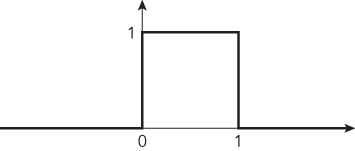
A distribution describes the relative likelihood of possible outcomes. In a uniform distribution (Figure 15-1), every outcome between the minimum and maximum possible outcome is equally likely. Naturally measured values like height often follow (or nearly follow) a Gaussian distribution (Figure 15-2), sometimes called a bell curve as its shape resembles a cross-section of a bell. The Gaussian distribution is so common that it is also called the normal distribution. Distributions can also be discrete. A classic example of this is the total number of heads you get when flipping a coin a given number of times. If you flip the coin n times, the relative probabilities of each possible total number of heads in the range of 0 to n is defined by a binomial distribution. When the number of outcomes of a discrete distribution becomes sufficiently large, it is often more convenient and fairly accurate to approximate it with a continuous distribution. For instance, for coin flips, as n increases beyond approximately 20, a Gaussian distribution becomes a good approximation to the binomial distribution.

Two key parameters of a distribution are the mean, which describes the central location of the distribution, and the variance, which describes the width of the distribution. The standard deviation is the square root of the variance.
Descriptive and Inferential Statistics
Descriptive statistics attempt to summarize some aspect of a data set; examples include the mean, median, and standard deviation. When a data set is a complete sample (includes all possible items), a statistic has a single value with no uncertainty. For instance, you might have a data set that includes the heights of all the employees in a company. From that, you could calculate the mean height of employees in the company. No matter how many times you repeat the process, you will get the same number. A statistic of a complete sample is a population statistic—in this case the population mean.
Most samples are incomplete (subsets of the population) because it would be difficult or impossible to obtain every possible value that could be in the data set. An unbiased, randomly selected set of values drawn from the complete population is called a representative sample. Statistics performed on a sample to try to understand the population on which the sample is based are called inferential statistics. A statistic calculated on a representative sample is called an estimate of the population statistic. These estimates always have associated uncertainty. Returning to the example of employee heights, if you didn’t have complete data on all employees in a large company, you might decide to collect heights on a random sample of 100 employees. The mean that you calculated from that sample would provide an estimate of the mean height of all employees (population mean). If you repeated the process with a different random sample, you would expect that you would get a slightly different value each time, because each sample would have different individuals in it. Each of the estimates of the mean would likely be close to but not exactly the same as the value of the population mean.
Confidence Intervals
The uncertainty in a sample statistic depends on the number of items in the sample (larger samples have less uncertainty) and the variance in the items being measured (larger variances yield greater uncertainty). A common measure of uncertainty of an estimate is a 95% confidence interval. A 95% confidence interval is defined as the interval such that if the process of constructing the sample and using it to calculate the interval were repeated a large number of times, 95% of the intervals would include that population statistic. So, if you took 1000 different samples of employee height data, you would calculate a slightly different sample mean and 95% confidence interval from each sample, and approximately 950 of these intervals would include the population mean height (the value you would calculate using data from all employees).
Statistical Tests
Statistical tests are used to compare estimates derived from samples to a given value (one sample test) or to the estimate from other samples (multiple sample tests). Most tests are constructed around the idea of a null hypothesis: that there is no difference in the population statistics being compared. The output of a test is a p-value. The p-value is the probability that, if the null hypothesis is true and there is actually no difference, the observed difference (or a larger difference) would occur by chance due to random sampling. Thus, the smaller the p-value, the less likely it is that the apparent difference based on the sample estimates is due to random chance, and the more likely it is that there is a true difference in the population(s).
It has become traditional to set the threshold at which a difference is considered “real” at p < 0.05. p-values below this threshold are commonly referred to as statistically significant. Although the 0.05 threshold has been imbued with an almost magical importance, it was arbitrarily selected. A rational application of statistics would involve considering the tolerance for uncertainty in the information that is sought with the test rather than blindly applying the conventional threshold.
While smaller p-values correspond to greater likelihood that a difference exists, it does not necessarily follow that larger p-values represent greater likelihood that there is no difference. A small p-value is evidence of likelihood of a difference, but absence of evidence of a difference is not evidence of no difference. The likelihood that a test will identify a difference when one exists is measured by the statistical power of the test; the p-value output by a test does not offer information about the statistical power. Failure of a test to identify a statistically significant difference can be interpreted as supporting absence of a difference greater than a given size only in the context of information about the statistical power of that test to detect a difference of the given size. Statistical power increases as sample size increases.
These principles can be illustrated with a concrete example. Suppose you wanted to determine whether there was a difference in average height between men and women at your company. You would start by determining the estimates of the mean heights based on two representative samples, one of men and one of women. A common statistical test that you might employ here is Student’s t-test, which compares estimates of means. You might assemble large samples of men and women, and observe a difference in estimates of the mean height of 5.1 inches. Applying a t-test might yield a p-value of 0.01. You would reasonably conclude that there is a statistically significant difference between mean heights of men and women in the company. You would be confident in this conclusion because the probability of observing the 5.1-inch (or greater) difference in mean heights between the two samples if the population mean heights of men and women were actually equal is 1%. A less motivated investigator might assemble small samples, observe a difference of 6 inches and obtain a p-value of 0.30 from a t-test. It would not be reasonable to conclude that there is a difference in mean heights from this data, because the probability that the observed difference could be due to chance with these small sample sizes is a relatively high 30%. Furthermore, assuming that the test was not well powered to detect a difference with the small sample sizes, it would not be reasonable to conclude that this result suggested that mean heights between men and women were the same. In this case, one could not reasonably draw any useful conclusions from this statistical test.
Every statistical test is based on assumptions about the data samples to which it is applied. For instance, the t-test assumes that sample data is drawn from a population that follows a Gaussian distribution. Tests that make assumptions about the distribution from which sample data is drawn are considered parametric statistics, while tests that do not make these assumptions are considered nonparametric statistics. Historically parametric statistics have been preferred because they have greater statistical power than equivalent nonparametric statistics at the same sample size (particularly when sample sizes are relatively small), and they are less computationally intensive. In the modern era, these advantages are often less relevant as computations are no longer done by hand, and differences in statistical power may be negligible when sample data set sizes are large.
Understanding the assumptions inherent in each statistical test or procedure, knowing how to determine whether or not those assumptions are violated, and using this knowledge to select the best statistics are the key characteristics of statistical expertise. Almost anyone can go through the steps of using statistical software to apply a test to a data set. This will yield a result regardless of whether the assumptions of the test have been violated, but the result may be meaningless if the assumptions are not true. A good statistician or data scientist is someone who can ensure that results are meaningful and interpret them usefully.
ARTIFICIAL INTELLIGENCE AND MACHINE LEARNING
Artificial intelligence (AI) is the discipline concerned with using computers to solve problems that require intelligence, similar to what most humans exhibit, rather than mere computation. Intelligence is a term that’s difficult to precisely define, and the border between computation and intelligence is subjective and difficult to delineate. While there is room for substantial debate about what is and is not included in artificial intelligence, there is general consensus that numerous tasks can be accomplished by a human using a computer, such as writing a book, that at present computers are unable to effectively accomplish on their own. Attempts to move toward autonomous solutions to those tasks and problems fall into the field of AI.
AI has a long and fascinating history of cyclical periods of breakthrough success leading to high expectations, followed by extended periods of disappointment at the failure of the breakthrough techniques to fully realize their promise. Although AI has repeatedly fallen short of its lofty goals, there have been substantial advances over the decades. One reason AI can appear to be a goal that is never attained is that the consensus opinion on where computation stops and AI starts is a moving target. Many problems that were once considered challenging AI goals, such as optical character recognition, games like chess or Go, voice recognition, and image classification, have now been largely solved. As people become accustomed to widespread computerized implementation of these techniques, they often cease to consider them to require intelligence.
To greatly oversimplify the complex history of AI, much of the early work in AI focused on explicitly representing knowledge in computational form and using formal logic and reasoning to make decisions and demonstrate intelligence. This had great success in limited domains, but frequently faltered in the face of attempts to address real-world data, which can be noisy, fragmentary, and internally inconsistent. The most recent successes and wave of enthusiasm for AI have been based largely on machine learning approaches. Although machine learning techniques have been around since the earliest days of AI, they have recently had great success in addressing problems that had been largely intractable with other AI approaches.
Machine learning techniques develop intelligence—the ability to make classifications or predictions—based on learning directly from data rather than being explicitly coded by humans. Machine learning is deeply rooted in statistics. For example, regression (fitting lines or curves to data) is both a fundamental statistical technique and commonly recognized as a simple form of machine learning. In machine learning the programmer writes code that defines the structure of the model, how it interacts with input data, and how it learns, but the intelligence and knowledge in the model is in the form of adjustable parameters that the model learns from training data. Machine learning can be supervised, in which each item of input data is paired with a desired output, and the goal is to learn how to reproduce the outputs based on the inputs; or unsupervised, in which case the goal is to learn outputs that represent commonalities between the inputs.
Machine learning includes a large family of techniques; much of the recent work in machine learning focuses on neural networks. In a neural network, processing occurs and knowledge is represented in connections between multiple layers of units that are loosely modeled on the function of neurons in the human brain. Neural networks themselves have a long history. The most recent iteration of neural network techniques is often referred to as deep learning. Deep learning is distinguished from earlier neural networks principally by a substantial increase in the number of layers in the network. The advent of successful deep learning has been driven by multiple factors, including the development of the Internet and cheap storage, which has made it feasible to assemble data sets large enough to train deep learning networks, and advancement of computational power, particularly GPU computation, which has made it possible to train large networks on large data sets in reasonable periods of time.
The process of machine learning starts with obtaining a sample data set. This data set must be representative of the data to which the model will eventually be applied; the model can’t learn anything that’s not in its training data.
Some preprocessing is typically performed on the data. Historically, this preprocessing was quite extensive, based on feature engineering: summary parameters of interest were extracted from the data based on algorithms designed by data scientists. The values extracted for these features then serve as the input to the machine learning model. Deep learning typically employs representation learning, in which the features are learned from the data rather than being explicitly coded. Representation learning has been particularly successful with natural world data like sound and images, where manual feature engineering has been exceptionally challenging. For representation learning, preprocessing is typically more minimal. For instance, preprocessing of an image data set might involve adjusting the pixel dimensions and average brightness to be the same for each image in the data set. The pixel values for each image then serve as the input to the machine learning model.
A data set is typically partitioned into a training set and a test set; the test set is kept separate and the model is trained using only the data in the training set. Most machine learning algorithms learn through an iterative process of examination of the training set. Ideally the performance of the model improves with each round of training until it converges: asymptotically approaches a theoretical maximum performance for the given model and training data set. For some machine learning techniques, including deep learning, it’s common to partition the data set into three parts: in addition to training and test, a validation set is used to monitor the progress of the training of the model. In addition to the parameters that the model learns from the data, many models have manually adjustable values that control the structure of the model (for example, the number of neurons in a layer) or aspects of how the model learns; these are referred to as hyperparameters. The converged model can then be run on the test set data to give an estimate of the expected performance on real-world data. Models typically perform better on the data that they’ve been directly exposed to in training; therefore, it’s important to keep the test set separate from the training set so that the performance estimate provided by the test set is unbiased.
RANDOM NUMBER GENERATORS
Random numbers are essential to a wide range of applications that work with or simulate real-world data. They are used in statistical analysis to facilitate construction of unbiased, representative samples. Random sampling is at the core of many machine learning algorithms. Games and simulations often lean heavily on random numbers, including for generating variety in scenarios and for the artificial intelligence procedures for non-player characters.
In interviews, random number generator problems combine mathematical concepts like statistics with computer code, allowing for evaluation of your analytical skills as well as your coding ability.
Most languages or standard libraries provide a random number generator. These functions are typically more properly referred to as pseudorandom number generators. A pseudorandom number generator produces a sequence of numbers that shares many properties with a true random sequence, but is generated by an algorithm employing deterministic calculations starting from one or more initial seed values. Because of the deterministic nature of the algorithm, a given algorithm will always produce the same sequence of “random” numbers when started with the same seed. Given a sufficiently long sequence of numbers from a pseudo-random generator, it may be possible to predict the next number in the sequence.
Truly random sequences (that is, nondeterministic sequences where the next number can never be predicted) cannot be created by any algorithm running on a standard CPU; they can only be generated by measuring physical phenomena that are inherently random, such as radioactive decay, thermal noise, or cosmic background radiation. Measuring these directly requires special hardware rarely found on general-purpose computers. Because some applications (notably cryptography) require the unpredictability of true randomness, many operating systems include random number generators that derive randomness from timing measurements of hardware found on typical computers, such as non–solid-state hard drives, keyboards, and mice.
Although hardware-based methods of random number generation avoid the deterministic predictability problems of pseudorandom number generators, they typically generate numbers at a much lower rate than pseudorandom number algorithms. When large quantities of unpredictable random numbers are needed, a hybrid approach is often employed, where a pseudorandom number generator is periodically reseeded using hardware-derived randomness. Depending on the requirements of the application, other methods may be used for seeding. For instance, a video game might seed the generator based on the system time, which would be insufficient to withstand a cryptographic attack, but sufficient to keep the game interesting by producing a different sequence every time the game is played. For debugging purposes, you might seed a generator with the same fixed value on every execution to improve the chances that bugs will be reproducible. Most libraries automatically seed their pseudorandom generators in some generally reasonable fashion, so you can usually assume in an interview that the random number generator is already seeded.
By convention, most random number generators produce sequences drawn from a standard uniform distribution (as seen in Figure 15-1); in other words, the generator function returns a value between 0 and 1, and every value between 0 and 1 has an equal likelihood of being returned. In typical implementations, this range is inclusive of 0 but exclusive of 1. Commonly, you may want random integers in a range between 0 and n. This is easily achieved by multiplying the value returned by the generator by n + 1 and taking the floor of this value.
DATA SCIENCE, RANDOM NUMBER AND STATISTICAL PROBLEMS
These problems require you to combine your knowledge of coding with understanding of mathematics, statistics and machine learning.
Irreproducible Results
You can imagine a wide variety of things that might have gone wrong here—the training and test data might not be representative of the actual data in production, for instance. There might be some error in how the models were implemented in production, or a difference in how data was preprocessed before being fed into the model. While you could speculate on any number of these possibilities, focus instead on the information given in the problem to identify something that’s definitely wrong.
Most of the information given focuses on the statistical test of model performance. You’re told that four of the hundred models tested have significantly better performance than random guessing. This means that 96 of the models can’t be distinguished from random guessing by this statistical test at a conventional threshold of significance; that’s nearly all of them. As a thought experiment, consider what you might expect the results to look like if all 100 of the models were in fact truly indistinguishable from random guessing.
Another way of putting that in statistical terms is to suppose that the null hypothesis were true for each model. You know from the definition of a p-value that if the null hypothesis is true, the p-value represents the probability that the difference observed in the test (in this case, the performance of the model) would occur by random chance. So with a p-value near 0.05, there’s approximately a 1 in 20 probability that what appears to be significant performance by the model is actually a fluke of randomness.
One in 20 is a fairly small probability, so if that were the probability of the well-performing models actually being useless then it would be possible but unlikely that the result was simply due to being unlucky. But is the probability of selecting a bad (equivalent to random guessing) model due to chance actually that low in this scenario?
You’re told that the statistical test is performed on the result of running each of the hundred models. So that means each one of the hundred models has a 1 in 20 chance of being selected as having statistically significant performance even if it in fact, does not. Because you’re testing 100 models, you would expect that if all 100 models were in fact worthless, about 5 would be identified as well-performing with p-values less than 0.05. (This expectation does assume that the performance of each of the models is independent of all of the other models. This is probably not entirely true if the models have some similarities and are trained on the same data, but as a first approximation it’s not unreasonable to assume independence.) This is essentially the scenario described in the problem, and this understanding resolves the apparent paradox between the test and real-world performance of these models.
You may recognize this as an example of a multiple testing problem. Put simply, the more things you look at and test, the higher the chances that at least one your tests will appear to be significant due to random chance. As a more concrete example, if someone told you they had a technique for rolling dice to get double sixes, you’d probably be impressed if they rolled once and got double sixes. If they rolled 50 times and got double sixes a couple of times you wouldn’t think they were doing anything special—that’s the outcome you’d expect.
When the real question is not whether a single result could be erroneously identified as significant due to chance, but whether any of a group of tests could be seen as significant due to chance, a multiple testing correction must be applied to the p-values to determine significance. The most common and widely known of these is the Bonferroni correction, wherein the p-value threshold is divided by the number of tests performed, and only tests with a p-value below this corrected threshold are considered significant. In this problem, this would yield a corrected threshold of 0.05/100 = 0.0005. None of the models have performance that differs from random guessing with p < 0.0005, so you would not identify any of them as having performance that is statistically significantly different from random guessing. The Bonferroni correction is very conservative: it errs strongly on the side of avoiding erroneously identifying differences as significant, and as a result may often fail to identify real differences, particularly when the multiple tests are not entirely independent. A wide variety of less conservative, generally more complex, corrections and multiple testing methods exist, but are beyond the scope of this book.
Multiple testing issues can be insidious and difficult to identify, because often the results of the few tests that met a threshold of significance are presented without the context of the many other non-significant tests that have been performed. For instance, the key to the problem presented here is knowing that 100 models were tested. Suppose that instead your colleagues told you only about the four models that did well in the tests and neglected to mention the 96 that failed. Understanding the poor real-world performance of these four models would be much more difficult. Presenting results as significant without acknowledging that they were selected from a large number of largely insignificant results is a deceitful practice referred to as data fishing, data dredging, or p-hacking.
Study More; Know Less
Ideally, improvements in performance on the training set are paralleled by improvements in performance on the validation set. When this desired behavior is seen, it is because both the training and validation data contain representative examples of the relationships between input and output data, and the model is learning these relationships. When performance between these sets diverges, it is because the model is learning something that is different between the two data sets. Assuming that both data sets are representative samples of the same population of data, the only difference between the two data sets is which specific items of data end up in each of the two sets. Logically then, when there is divergence in performance between training and validation data sets, it is often because the model is learning about the specific items of data in the training data set rather than the underlying structure of the data that these items illustrate.
This problem is called overfitting. Overfitting occurs when there is insufficient training data relative to the number of parameters for which the model is trying to learn values. In this situation, the model can achieve optimal performance on training data by using the parameters of the model to effectively memorize the correct output for each of the items in the training data set. If there were more training data or fewer parameters in the model, then the model wouldn’t have sufficient capacity to memorize each item in the training set. Because it couldn’t achieve good performance by memorizing inputs, the learning process would force it to identify a smaller number of aspects of the structure of the underlying data to achieve good performance. This is what you want, because these structural aspects of the data are generalizable outside of the training set.
As a more concrete example of this, you might find that your overfitted model has learned to connect something that uniquely identifies each player in your training set with whether or not that player is cheating, but that these things that it has learned are irrelevant to the issue of cheating. For instance, it might learn that the player who starts on top of the castle and immediately descends into the dungeon is a cheater, while the player who starts in the southeast corner of the woods is not a cheater. This kind of memorization leads to exceptionally high performance on the training data. Because the things that are learned have nothing to do with whether or not a player is cheating (a cheating player could just as easily start in the woods), the model has very poor performance outside of the training set that it has memorized. A model that was not overfitted might instead learn that players who have successive locations that are far apart (representing travel faster than allowed by the game) are cheaters—this would likely produce good performance that is generalizable outside of the training set.
Because overfitting is typically a consequence of having too many parameters relative to the amount of training data, two general solutions are to increase the amount of training data or to decrease the number of parameters to be learned.
In general the ideal solution to overfitting is to increase the amount of training data, but frequently it is either impossible or too expensive to be feasible to increase the size of the training data set sufficiently to resolve the overfitting. In some cases it may be possible to effectively increase the size of the input data set by algorithmically making random perturbations of the input data. This process is called augmentation. It is particularly useful for representation learning, as often multiple straightforward perturbation algorithms can be selected. For instance, if you were using machine learning for image recognition, you might augment your input data set by performing multiple random rotations, translations, and/or scaling on each input image. Intuitively this makes sense: if you want the model to learn to recognize sailboats, you don’t want it to learn the specific location and pixel size of the sailboats in the training data set, you want it to learn to recognize sailboats generally, at any location, size, or rotation within the image.
Another approach is to decrease the number of parameters available to the model. (Note that “number of parameters” here actually refers to a combination of the actual number of parameters and the flexibility of the model in employing those parameters, since two different models with different structures and the same absolute number of parameters may have differing degrees of proclivity to overfitting.) Ways to accomplish this include changing the type of machine learning approach you’re using to something simpler, or maintaining the same approach but changing something structural about the model to decrease the number of parameters. For instance, deep learning networks for image recognition commonly downsample the images to low resolution as part of the preprocessing (256 × 256 pixels is common). A major reason for this is that each pixel represents additional inputs to the model and requires additional parameters, so using low-resolution images reduces the number of parameters and helps to avoid overfitting. A drawback to avoiding overfitting by reducing parameters is that the resulting models have less descriptive power, so they may not be able to recognize all the aspects of the data that you would like them to.
Several other techniques can be used to try to avoid overfitting without reducing the number of parameters. When the learning process is iterative, models often move through an early period of learning the generalizable structure of the underlying data and then begin to overfit on specific aspects of items in the training data set. Early stopping attempts to avoid overfitting by choosing the optimum point to stop learning—after most of the generalizable structure has been learned but before too much overfitting has occurred.
Another approach to dealing with limited training data that’s particularly important for deep learning is transfer learning. Transfer learning is based on the observation that well-performing learned parameter sets for models that do similar things tend to be similar. For instance, there is substantial similarity between most well-performing image recognition neural networks, even if they’re trained to recognize different objects. Suppose that you want to develop a model to recognize images of different kinds of electronic components, but (even using augmentation) you don’t think you have a sufficient number of images in your training set to avoid overfitting and develop a well-performing generalizable model. Instead of starting by initializing the parameters in your model to random values, you could employ transfer learning by using a pretrained network as your starting point. (Networks trained on ImageNet, a very large collection of categorized images, are widely available and commonly used for transfer learning.) Then you retrain the network using your electronic component images. Typically during this retraining, only some of the parameters from the pretrained network are allowed to change and/or hyperparameters are set to limit the extent to which parameters can change. This has the effect of reducing the number of parameters to be learned from your training data set, reducing problems with overfitting, without requiring oversimplification of the model. The outcome is usually a model that performs substantially better than what could be achieved using a small training data set alone.
Roll the Dice
The output of this function will be two numbers, each in the range of 1 to 6, inclusive (because each die has six sides). Each time the function is called, it will likely yield different results, just like rolling a pair of dice.
Recall that most random number generators yield a floating-point number between 0 and 1. The primary task in implementing this function is to transform a floating point in the range of 0 to 1 into an integer in the range of 1 to 6. Expanding the range is easily accomplished by multiplying by 6. Then you need to convert from floating point to an integer. You might consider rounding the result; what would that produce? After multiplication, you’ll have a value r such that 0 ≤ r < 6. Rounding this result would yield an integer in the range 0 to 6, inclusive. That’s seven possible values, which is one more than you want. Additionally, this process is twice as likely to yield a value in the range 1 to 5 as it is a 0 or 6, because, for example, the portion of the range of r that rounds to 1 is twice as wide as the portion that rounds to 0. Alternatively, if you use floor to truncate the fractional part of r, you’ll end up with one of six possible values 0 to 5, each with equal probability. That’s almost what you need. Just add 1 to get a range of 1 to 6, and then print the result. Do this twice, once for each die.
We’ll implement this function in JavaScript:
function rollTheDice() {var die1 = Math.floor(Math.random() * 6 + 1);var die2 = Math.floor(Math.random() * 6 + 1);console.log("Die 1: " + die1 + " Die 2: " + die2);}
Random number generation is relatively computationally expensive, so the execution time of this function is dominated by the two RNG calls.
This is a little more challenging. When you roll the first die, you get one of six possibilities. When you roll the second die, you again get one of six possibilities. This creates 36 total possible outcomes for a roll of two dice. You could write out all 36, starting at 1-1, 1-2…6-5, 6-6; keep in mind that order is important, so for instance 2-5 is different from 5-2. You could use this enumeration of outcomes to simulate the pair of dice by generating a random number in the range of 1–36 and mapping each of these values to one of the possible outcomes using a switch statement. This would work, but would be somewhat inelegant.
Instead, how could you take a number in the range of 1–36, and transform it into two numbers, each in the range of 1–6?
One possibility is to integer divide the number by 6. This would give you one number between 0 and 6, but unfortunately the outcomes wouldn’t be equally likely. You would get a 6 only 1/36 of the time, when the random number was 36.
You need to select an initial range where each outcome will be equally likely. If you take a random number in the range 0–35, and integer divide by 6 you get six equally likely outcomes between 0 and 5. If you take modulo 6 of the random number you get six additional independent equally likely outcomes between 0 and 5. You can add 1 to each of these to transform from the 0-based world of code to the 1-based world of dice.
JavaScript doesn’t have an integer divide operator (the result is always a floating point), so you have to perform a floor operation after the divide to achieve the desired result. The resulting code looks like:
function rollTheDice() {var rand0to35 = Math.floor(Math.random() * 36);var die1 = Math.floor(rand0to35 / 6) + 1;var die2 = (rand0to35 % 6) + 1;console.log("Die 1: " + die1 + " Die 2: " + die2);}
This is almost twice as fast as the previous implementation because it makes only one call to the RNG.
Take these one at a time.
The first function is pretty straightforward. You just need to split the six outcomes of dieRoll() into two groups of three and map each of these to the two outcomes you want (1 or 2). For instance, you can return 1 if the random number is 1–3 and 2 if it isn’t. Other possibilities exist, such as modulo 2.
Implementing in JavaScript yields:
function dieRoll2() {var die2;var die6 = dieRoll();if (die6 <= 3) {die2 = 1;} else {die2 = 2;}return die2;}
dieRoll3() could be implemented the same way: split the range into subranges of 1–2, 3–4, and 5–6 representing 1, 2, or 3, respectively. Alternatively, you could use some other way to divide the six numbers into equal groups, such as modulo by 3 (and adding 1) or dividing by 2. Dividing by two produces a concise solution. The only tricky part is remembering to take the ceiling of the number (since the odd numbers will yield fractional parts, which need to be rounded up):
function dieRoll3() {var die3;var die6 = dieRoll();die3 = Math.ceil(die6 / 2);return die3;}
dieRoll4() is a little tougher, because 6 does not divide evenly into four parts. You may be tempted to roll the die twice and sum the numbers to get an answer between 2 and 12, since 12 is divisible by 4. However, this answer would be difficult to work with, because the numbers would not be evenly distributed. Several rolls can sum to 7, but 2 and 12 can each be produced by only one roll.
Consider whether you can use one of the functions you’ve already implemented, dieRoll2() or dieRoll3(). dieRoll2() effectively gives you a random bit. You can create two bits by calling it twice. Putting these together into a two-digit binary number yields a value 0-3, to which you can add one for the desired result. Another way to think of this is that if you call dieRoll2() twice, you have four possible outcomes—1-1, 1-2, 2-1, and 2-2:
function dieRoll4(){var die4;die2First = dieRoll2() - 1;die2Second = dieRoll2() - 1;die4 = (die2First * 2 + die2Second) + 1;return die4;}
The strategies that worked well for the other functions don’t apply to dieRoll5 because 5 is neither a factor of 6 nor a multiple of one of the other numbers you’ve worked out.
You’re going to need a new approach for this problem. Try reconsidering the core problem: use a six-sided die to produce a number in the range 1–5. What else could you do with the result of the die roll? Reconsider the assumptions. One of the assumptions has been that each of the six possible outcomes of the die has to be mapped in some way to an outcome in the desired smaller range. Is that really necessary?
If you just ignored one of the outcomes of the die roll, that would give you five equally likely outcomes, which is exactly what you’re looking for. But suppose you “ignore” 6—what do you do when dieRoll() returns a 6? If you know how to play craps, that may give you an idea. In craps, after the first roll, if the dice come up as anything other than the target number (the point) or 7, the outcome is ignored by rolling again. You could apply this strategy to the current situation by accepting any number in the range 1–5 and ignoring 6 by rerolling. If you got another 6 you would reroll again. In theory this could go on forever, but since the probability of rolling n consecutive 6’s is 6-n, which rapidly becomes very small as n increases, it’s extremely unlikely that this would go on very long.
In summary, you roll the die, and if you get an outcome 1–5, you accept the number. If you get a 6, you call dieRoll() again to reroll.
This answer looks like:
function dieRoll5() {var die5;do {die5 = dieRoll();} while (die5 == 6);return die5;}
This is an example of a problem where you may feel stuck, because the strategies that were successful for similar problems don’t work. Once you realize that you can ignore some outcomes by rerolling, the solution is quite simple. In fact, this method would also work (though less efficiently) for dieRoll2(), dieRoll3(), and dieRoll4(). When you get stuck, remember to return to the original problem and assess your assumptions to identify a new approach.
Calculate Pi
You’re given so little in this problem that it may be hard to see where to start. If you don’t have experience with Monte Carlo methods, the requirements of this problem may seem nonsensical. You need to calculate π, which always has the same, fixed value, but you need to do so using an RNG, which is inherently random.
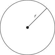
Start by thinking about what you know about π. First, you know that in a circle, c = πd, where circumference is c and diameter is d. You also know that the area of a circle with radius r is πr2. That’s a start. Sort of a middle school math start, but still a start.
Try drawing a picture (Figure 15-3)—that often helps when an answer is not obvious initially.
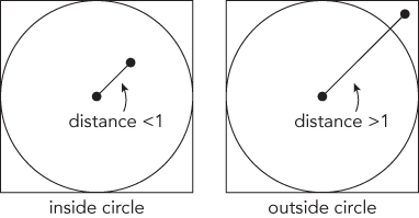
You have a circle. What else do you have? You have a random number generator. What can you do with an RNG? The random numbers that you generate could be radii for randomly sized circles, or you could create points randomly. Randomly selected points might fall inside or outside of the circle. How might you be able to use randomly generated points that are inside the circle or outside the circle? Add some points to your drawing, as in this picture with two points, one inside and one outside (Figure 15-4).

In this drawing, we have a point inside, and a point outside. Because both coordinates of the point are drawn from a uniform distribution, every point within the range over which you are choosing points has an equal probability of being selected. Put another way, the probability of a point being found in any particular region is proportional to the area of that region. What is the probability of a random point being inside the circle? To make it easy, make the radius of the circle 1 and choose each coordinate of the random point to be between –1 and 1. What’s the probability of a point being inside the circle? The area of the circle is πr2. And the area of the square around the circle is 2r * 2r = 4r2. So the likelihood of a point being in the circle is

Because the probability of any one point being inside the circle is π / 4, if you randomly select and test a large number of points, approximately π / 4 of them will be inside the circle. If you multiply that ratio by 4 you have an approximation of π.
That’s exactly what you were looking for, but there’s one more step—how do you know if a point is inside the circle or outside the circle? The definition of a circle is the set of all points equidistant from the center. In this case, any point that has a distance of 1 or less from the center, as in Figure 15-5, is inside the circle.
Now you just need to determine the distance of a point from the center of the circle, which is located at (0,0). You know the x and the y values of the point, so you can use the Pythagorean Theorem, x2 + y2 = z2, where z is the distance from the center of the circle. Solving for z, ![]() , the point is in the circle. If z > 1, the point is outside of the circle. You don’t care about the actual distance from the center, only whether or not it is greater than 1, so you can optimize slightly by eliminating the square root. (This works because every number greater than 1 has a square root greater than 1 and every number less than or equal to 1 has a square root less than or equal to 1.) As an additional simplification, you can work with only the upper-right quadrant of the circle, choosing points where both coordinates are in the range 0–1. This eliminates ¾ of the square and ¾ of the circumscribed circle, so the ratio remains the same.
, the point is in the circle. If z > 1, the point is outside of the circle. You don’t care about the actual distance from the center, only whether or not it is greater than 1, so you can optimize slightly by eliminating the square root. (This works because every number greater than 1 has a square root greater than 1 and every number less than or equal to 1 has a square root less than or equal to 1.) As an additional simplification, you can work with only the upper-right quadrant of the circle, choosing points where both coordinates are in the range 0–1. This eliminates ¾ of the square and ¾ of the circumscribed circle, so the ratio remains the same.
Putting this all together as pseudocode:
loop over number of iterationsgenerate a random point between (0,0) and (1,1)if distance between (0,0) and the point is <=1increment counter of points inside circleend loopreturn 4 * number of points inside circle / number of iterations
Now, write the code. In JavaScript, it might look like:
function estimatePi(iterations) {var i;var randX;var randY;var dist;var inside = 0;for (i = 0; i < iterations; i++) {randX = Math.random();randY = Math.random();dist = (randX * randX) + (randY * randY);if (dist <= 1) {inside++;}}return (4 * (inside / iterations));}
As a test, one execution of this function using a value of 100,000,000 for iterations returned an estimate of 3.14173 for π, which matches the true value of 3.14159… to several decimal places.
The solution to this problem is a classic example of a simple application of the Monte Carlo method. Monte Carlo methods use randomly generated inputs to solve problems. They are often useful when a result for a single input can be calculated relatively quickly, but the value of interest is based on some aggregation of all or many possible inputs.
If you’ve worked with Monte Carlo methods before, there’s a good chance you’ve seen the solution to this problem as an introductory example. If not, this may be a fairly challenging problem, because you essentially have to rediscover Monte Carlo methods along the way. Nevertheless, based on what’s in the problem statement and a few geometrical facts, it’s something you can work through to discover an interesting application for a random number generator.
Intuitively, you probably know that as you increase the number of iterations, the estimate that you calculate is likely to become closer to the true value of π. Based on this, your first inclination might be to determine this empirically: try estimating π with several different levels of numbers of iterations and compare the results. This would probably get you in the ballpark of the right answer fairly quickly, and for some applications that might be sufficient. However, refining that solution to get a precise value for minimum required number of iterations could start to require quite a bit of computation. For any given number of iterations, you would need to repeat the process of estimating π many times in order to get an accurate estimate of what percentage of the estimates were within 0.01 of the true value. Furthermore, you would likely have to repeat that whole procedure for many different values of the number of iterations. While simple in concept, getting an accurate solution using this approach seems like it could require a lot of work and a lot of computer power.
Instead, consider whether there’s an analytic approach you can take to solving this problem using what you know about statistics.
Because the estimation method is based on a random number generator, each time you perform it (starting from a different seed value) you’ll get a somewhat different value for your estimate of π, even when using the same number of iterations. Another way to put this is that there is a distribution of the estimates around the true value of π. The wider this distribution is, the fewer of the estimates there will be that are within 0.01 of the true value of π. In order for there to be a 95% chance of the estimate being within 0.01 of the true value of π, you need to find the number of iterations that produces a distribution of estimates where 95% of the distribution is within 0.01 of π.
What distribution do the estimates of π follow? Consider the procedure you’re using to estimate the value of π. Each randomly selected point either does or does not fall within the circle—these are the only two possibilities. So you have multiple repetitions of a random event that has only two possible outcomes. This sounds very much like a series of coin flips, with the only difference being that the probabilities of the two outcomes are not equal. Just as for coin flips, the number of points within the circle follows a binomial distribution. If you have experience with statistics you may recall that the two parameters that define a binomial distribution are n, the number of random events (in this case, the number of iterations) and p, the probability of any event being a “success” (in this case, inside the circle). You know the probability that a point will be inside the circle, so p = π/4. You need to find the value of n that produces a binomial distribution of the appropriate width for this value of p.
Binomial distributions are difficult to work with, especially as n becomes large, but as n becomes large they are well approximated by a normal distribution having the same mean and standard deviation. The mean of a binomial distribution is np and the standard deviation is ![]() . Remember that these are the parameters for the distribution of the number of points inside the circle. You divide that by the number of iterations and multiply by 4 to obtain the estimate of π, so you need to do the same thing to the distribution to obtain the distribution of the estimates of π.
. Remember that these are the parameters for the distribution of the number of points inside the circle. You divide that by the number of iterations and multiply by 4 to obtain the estimate of π, so you need to do the same thing to the distribution to obtain the distribution of the estimates of π.
Doing so for the mean gives np(4/n) = 4p = 4(π/4) = π which provides reassurance that you’ve correctly defined the parameters for this distribution. For the standard deviation, you have ![]()
![]()
At this point, you’ve defined the distribution of the estimates of the value of π, and you know the mean and standard deviation. You need the value of n such that 95% of this distribution will fall within 0.01 of π. The mean of the distribution is π. You may recall that for a normal distribution 95% of the distribution falls within a range of approximately ±1.96 standard deviations centered on the mean. This piece of information completes your equation:

Solving for n: n = 1962(4 – π) π. Using the known value for π, this is equal to about 104,000.
You may have noted that there’s a little circularity in this solution. The goal of the whole process is to determine a value for π, but you need a value for π to determine how many points are needed for a given level of accuracy in π. You could address this by choosing an arbitrary number of points for an initial estimate of π, use that estimated value of π to determine how many points you need for an estimate of π with the required precision, and then repeat the estimation process using that number of points to yield a value of π that you could use in the preceding equation.
SUMMARY
Statistics is the branch of mathematics that deals with chance and uncertainty. Randomness is inherent in chance and uncertainty, and random number generators are the principal source of randomness on computers. Although historically most programmers have not needed to have much knowledge in these areas, the machine learning approaches that are currently showing the most promise in developing artificial intelligence solutions to dealing with real-world data are strongly rooted in statistics. A new field of data science is emerging at the interface between computer science and statistics. If you want to embrace this field and become a data scientist, you need to develop skills in statistics and machine learning equal to your expertise in programming. Even if you expect to remain in more traditional areas of coding and programming, machine learning techniques seem likely to have increasingly wide application, so it’s worthwhile to develop some understanding of data science, random numbers, and statistics.