14

Profiling

It is quite common that written code doesn't behave perfectly after being tested with real data. Other than bugs, we can find the problem that the performance of the code is not adequate. Perhaps some requests are taking too much time, or perhaps the usage of memory is too high.

In those cases, it's difficult to know exactly what the key elements are, that are taking the most time or memory. While it's possible to try to follow the logic, normally once the code is released, the bottlenecks will be at points that are almost impossible to know beforehand.

To get information on what exactly is going on and follow the code flow, we can use profilers to dynamically analyze the code and better understand how the code is executed, in particular, where most time is spent. This can lead to adjustments and improvements affecting the most significant elements of the code, driven by data, instead of vague speculation.

In this chapter, we'll cover the following topics:

• Profiling basics
• Types of profilers
• Profiling code for time
• Partial profiling
• Memory profiling

First, we will take a look at the basic principles of profiling.

Profiling basics

Profiling is a dynamic analysis that instruments code to understand how it runs. This information is extracted and compiled in a way that can be used to get a better knowledge of a particular behavior based on a real case, as the code is running as usual. This information can be used to improve the code.

The normal application of profiling is to improve the performance of the code under analysis. By understanding how it executes in practice, it sheds light on the dynamics of the code modules and parts that could be causing problems. Then, actions can be taken in those specific areas.

Performance can be understood in two ways: either time performance (how long code takes to execute) or memory performance (how much memory the code takes to execute). Both can be bottlenecks. Some code may take too long to execute or use a lot of memory, which may limit the hardware where it's executed.

A common case in software development is that you don't really know what your code is going to do until it gets executed. Clauses to cover corner cases that appear rare may execute much more than expected, and software works differently when there are big arrays, as some algorithms may not be adequate.

The problem is that doing that analysis before having the system running is incredibly difficult, and at most times, futile, as the problematic pieces of code will very likely be completely unexpected.

Programmers waste enormous amounts of time thinking about, or worrying about, the speed of noncritical parts of their programs, and these attempts at efficiency actually have a strong negative impact when debugging and maintenance are considered. We should forget about small efficiencies, say about 97% of the time: premature optimization is the root of all evil. Yet we should not pass up our opportunities in that critical 3%.

Donald Knuth – Structured Programing with GOTO Statements - 1974.

Profiling gives us the ideal tool to not prematurely optimize, but to optimize according to real, tangible data. The idea is that you cannot optimize what you cannot measure. The profiler measures so it can be acted upon.

Profiling can be achieved in different ways, each with its pros and cons.

Types of profilers

There are two main kinds of time profilers:

• Deterministic profilers, through a process of tracing. A deterministic profiler instruments the code and records each individual command. This makes deterministic profilers very detailed, as they can follow up the code on each step, but at the same time, the code is executed slower than without the instrumentation.
• Deterministic profilers are not great to execute continuously. Instead, they can be activated in specific situations, like while running specific tests offline, to find out problems.
• Statistical profiles, through sampling. This kind of profiler, instead of instrumenting the code and detecting each operation, awakes at certain intervals and takes a sample of the current code execution stack. If this process is done for long enough, it captures the general execution of the program.

While they don't give as detailed information as deterministic profiles, statistical profilers are much more lightweight and don't consume many resources. They can be enabled to constantly monitor live systems without interfering with their performance.

Statistical profilers only make sense on systems that are under relative load, as in a system that is not stressed, they'll show that most time is spent waiting.

Statistical profilers can be internal, if the sampling is done directly on the interpreter, or even external if it's a different program that is taking the samples. An external profiler has the advantage that, even if there's any problem with the sampling process, it won't interfere with the program being sampled.

Both profilers can be seen as complementary. Statistical profilers are good tools for understanding the most-visited parts of the code and where the system, aggregated, is spending time. They live in the live system, where the real case usages determine the behavior of the system.

The deterministic profilers are tools for analyzing specific use cases in the petri dish of the developer's laptop, where a specific task that is having some problem can be dissected and analyzed carefully, to be improved.

Typically, code will present hotspots, slow parts of it that get executed often. Finding the specific parts to focus attention on and then act on them is a great way to improve the overall speed.

These hotspots can be revealed by profiling, either by checking the global hotspots using a statistical profiler or the specific hotspots for a task with a deterministic profiler. The first will display the specific parts of the code that are most used in general, which allows us to understand the pieces that get hit more often and take the most time in aggregate. The deterministic profiler can show, for a specific task, how long it takes for each line of code, and determine what are the slow elements.

Another kind of profiler is the memory profiler. A memory profiler records when memory is increased and decreased, tracking the usage of memory. Profiling memory is typically used to find out memory leaks, which are rare for a Python program, but they can happen.

Python has a garbage collector that releases memory automatically when an object is not referenced anymore. This happens without having to take any action, so compared with programs with manual memory assignment, like C/C++, the memory management is easier to handle. The garbage collection mechanism used for Python is called reference counting, and it frees memory immediately once a memory object is not used by anyone, as compared with other kinds of garbage collectors that wait.

In the case of Python, memory leaks can be created by three main use cases, from more likely to least:

• Some objects are still referenced, even if they are not used anymore. This can typically happen if there are long-lived objects that keep small elements in big elements, like lists of dictionaries when they are added and not removed.
• An internal C extension is not managing the memory correctly. This may require further investigation with specific C profiling tools, which is out of scope for this book.
• Complex reference cycles. A reference cycle is a group of objects that reference each other, e.g. object A references B and object B references A. While Python has algorithms to detect them and release the memory nonetheless, there's the small possibility that the garbage collector is disabled or any other bug problem. You can see more information on the Python garbage collector here: https://docs.python.org/3/library/gc.html.

The most likely situation for extra usage of memory is an algorithm that uses a lot of memory, and detecting when the memory is allocated can be achieved with the help of a memory profiler.

Let's introduce some code and profile it.

Profiling code for time

We will start by creating a short program that will calculate and display all prime numbers up to a particular number. Prime numbers are numbers that are only divisible by themselves and one.

We will start by taking a naïve approach first:

def check_if_prime(number):
    result = True
    for i in range(2, number):
        if number % i == 0:
            result = False
    return result

This code will take every number from 2 to the number under test (without including it), and check whether the number is divisible. If at any point it is divisible, the number is not a prime number.

To calculate all the way from 1 to 5,000, to verify that we are not making any mistakes, we will include the first prime numbers lower than 100 and compare them. This is on GitHub, available as primes_1.py at https://github.com/PacktPublishing/Python-Architecture-Patterns/blob/main/chapter_14_profiling/primes_1.py.

PRIMES = [1, 2, 3, 5, 7, 11, 13, 17, 19, 23, 29, 31, 37, 41, 43, 47, 53,
          59, 61, 67, 71, 73, 79, 83, 89, 97]
NUM_PRIMES_UP_TO = 5000
def check_if_prime(number):
    result = True
    for i in range(2, number):
        if number % i == 0:
            result = False
    return result
if __name__ == '__main__':
    # Calculate primes from 1 to NUM_PRIMES_UP_TO
    primes = [number for number in range(1, NUM_PRIMES_UP_TO)
              if check_if_prime(number)]
    # Compare the first primers to verify the process is correct
    assert primes[:len(PRIMES)] == PRIMES
    print('Primes')
    print('------')
    for prime in primes:
        print(prime)
    print('------')

The calculation of prime numbers is performed by creating a list of all numbers (from 1 to NUM_PRIMES_UP_TO) and verifying each of them. Only values that return True will be kept:

    # Calculate primes from 1 to NUM_PRIMES_UP_TO
    primes = [number for number in range(1, NUM_PRIMES_UP_TO)
              if check_if_prime(number)]

The next line asserts that the first prime numbers are the same as the ones defined in the PRIMES list, which is a hardcoded list of the first primes lower than 100.

assert primes[:len(PRIMES)] == PRIMES

The primes are finally printed. Let's execute the program, timing its execution:

$ time python3 primes_1.py
Primes
------
1
2
3
5
7
11
13
17
19
… 
4969
4973
4987
4993
4999
------
Real      0m0.875s
User      0m0.751s
sys 0m0.035s

From here, we will start analyzing the code to see what is going on internally and see if we can improve it.

Using the built-in cProfile module

The easiest, faster way of profiling a module is to directly use the included cProfile module in Python. This module is part of the standard library and can be called as part of the external call, like this:

$ time python3 -m cProfile primes_1.py
Primes
------
1
2
3
5
...
4993
4999
------
         5677 function calls in 0.760 seconds
   Ordered by: standard name
   ncalls  tottime  percall  cumtime  percall filename:lineno(function)
        1    0.002    0.002    0.757    0.757 primes_1.py:19(<listcomp>)
        1    0.000    0.000    0.760    0.760 primes_1.py:2(<module>)
     4999    0.754    0.000    0.754    0.000 primes_1.py:7(check_if_prime)
        1    0.000    0.000    0.760    0.760 {built-in method builtins.exec}
        1    0.000    0.000    0.000    0.000 {built-in method builtins.len}
      673    0.004    0.000    0.004    0.000 {built-in method builtins.print}
        1    0.000    0.000    0.000    0.000 {method 'disable' of '_lsprof.Profiler' objects}
Real      0m0.895s
User      0m0.764s
sys 0m0.032s

Note this called the script normally, but also presented the profile analysis. The table shows:

• ncalls: Number of times each element has been called
• tottime: Total time spent on each element, not including sub calls
• percall: Time per call on each element (not including sub calls)
• cumtime: Cumulative time – the total time spent on each element, including subcalls
• percall: Time per call on an element, including subcalls
• filename:lineno: Each of the elements under analysis

In this case, the time is clearly seen to be spent in the check_if_prime function, which is called 4,999 times, and it takes the practical totality of the time (744 milliseconds compared with a total of 762).

While this text table can be enough for simple scripts like this one, the output can be presented as a file and then displayed with other tools:

$ time python3 -m cProfile -o primes1.prof  primes_1.py
$ ls primes1.prof
primes1.prof

Now we need to install the visualizer SnakeViz, installing it through pip:

$ pip3 install snakeviz

Finally, open the file with snakeviz, which will open a browser with the information:

$ snakeviz primes1.prof
snakeviz web server started on 127.0.0.1:8080; enter Ctrl-C to exit
http://127.0.0.1:8080/snakeviz/%2FUsers%2Fjaime%2FDropbox%2FPackt%2Farchitecture_book%2Fchapter_13_profiling%2Fprimes1.prof

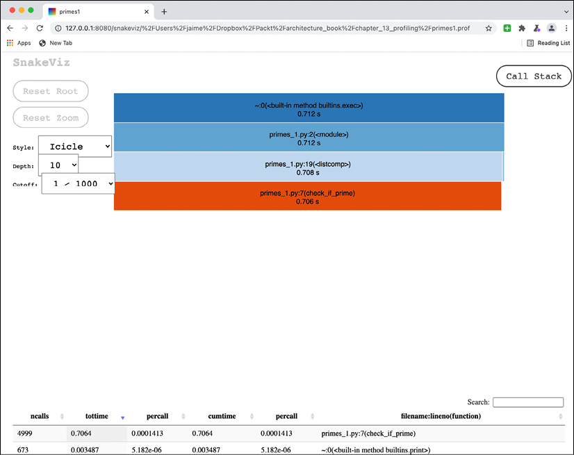
Figure 14.1: Graphical representation of the profiling information. The full page is too big to fit here and has been cropped purposefully to show some of the info.

This graph is interactive, and we can click and hover on different elements to get more information:

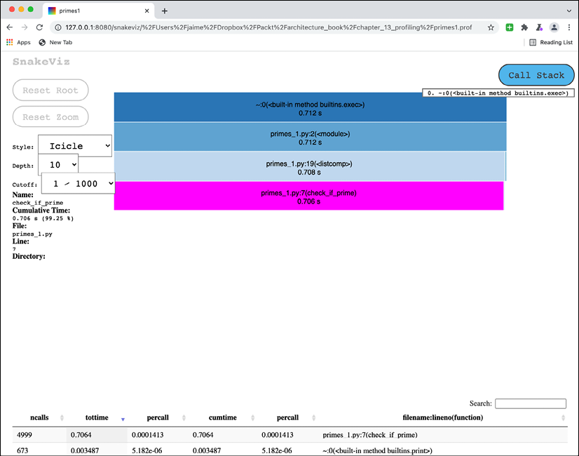
Figure 14.2: Checking the information about check_if_prime. The full page is too big to fit here and has been cropped purposefully to show some of the info.

We can confirm here that the bulk of the time is spent on check_if_prime, but we don't get information about what's inside it.

This is because cProfile only has function granularity. You'll see how long each function call takes, but not a lower resolution. For this specifically simple function, this may not be enough.

We will see how to use a profiler that has a higher resolution, analyzing each line of code.

Line profiler

To analyze the check_if_prime function, we need to first install the module line_profiler

$ pip3 install line_profiler

After it's installed, we will make a small change in the code, and save it as primes_2.py. We will add the decorator @profile for the check_if_prime function, to indicate to the line profiler to look into it.

The code will be like this (the rest will be unaffected). You can check the whole file on GitHub at https://github.com/PacktPublishing/Python-Architecture-Patterns/blob/main/chapter_14_profiling/primes_2.py.

@profile
def check_if_prime(number):
    result = True
    for i in range(2, number):
        if number % i == 0:
            result = False
    return result

Execute the code now with kernprof, which will be installed after the installation of line_profiler.

$ time kernprof -l primes_2.py
Primes
------
1
2
3
5
…
4987
4993
4999
------
Wrote profile results to primes_2.py.lprof
Real      0m12.139s
User      0m11.999s
sys 0m0.098s

Note the execution took noticeably longer – 12 seconds compared with subsecond execution without the profiler enabled. Now we can take a look at the results with this command:

$ python3 -m line_profiler primes_2.py.lprof
Timer unit: 1e-06 s
Total time: 6.91213 s
File: primes_2.py
Function: check_if_prime at line 7
Line #      Hits         Time  Per Hit   % Time  Line Contents
==============================================================
     7                                           @profile
     8                                           def check_if_prime(number):
     9      4999       1504.0      0.3      0.0      result = True
    10
    11  12492502    3151770.0      0.3     45.6      for i in range(2, number):
    12  12487503    3749127.0      0.3     54.2          if number % i == 0:
    13     33359       8302.0      0.2      0.1              result = False
    14
    15      4999       1428.0      0.3      0.0      return result

Here, we can start analyzing the specifics of the algorithm used. The main problem seems to be that we are doing a lot of comparisons. Both lines 11 and 12 are being called too many times, though the time per hit is short. We need to find a way to reduce the number of times they're being called.

The first one is easy. Once we find a False result, we don't need to wait anymore; we can return directly, instead of continuing with the loop. The code will be like this (stored in primes_3.py, available at https://github.com/PacktPublishing/Python-Architecture-Patterns/blob/main/chapter_14_profiling/primes_3.py):

@profile
def check_if_prime(number):
    for i in range(2, number):
        if number % i == 0:
            return False
    return True
Let's take a look at the profiler result.
$ time kernprof -l primes_3.py
... 
Real      0m2.117s
User      0m1.713s
sys       0m0.116s
$ python3 -m line_profiler primes_3.py.lprof
Timer unit: 1e-06 s
Total time: 0.863039 s
File: primes_3.py
Function: check_if_prime at line 7
Line #      Hits         Time  Per Hit   % Time  Line Contents
==============================================================
     7                                           @profile
     8                                           def check_if_prime(number):
     9
    10   1564538     388011.0      0.2     45.0      for i in range(2, number):
    11   1563868     473788.0      0.3     54.9          if number % i == 0:
    12      4329       1078.0      0.2      0.1              return False
    13
    14       670        162.0      0.2      0.0      return True

We see how time has gone down by a big factor (2 seconds compared with the 12 seconds before, as measured by time) and we see the great reduction in time spent on comparisons (3,749,127 microseconds before, and then 473,788 microseconds), mainly due to the fact there are 10 times fewer comparisons, 1,563,868 compared with 12,487,503.

We can also improve and further reduce the number of comparisons by limiting the size of the loop.

Right now, the loop will try to divide the source number between all the numbers up to itself. For example, for 19, we try these numbers (as 19 is a prime number, it's not divisible by any except for itself).

Divide 19 between
[2, 3, 4, 5, 6, 7, 8, 9, 10, 11, 12, 13, 14, 15, 16, 17, 18, 19]

Trying all these numbers is not necessary. At least, we can skip half of them, as no number will be divisible by a number higher than half itself. For example, 19 divided by 10 or higher is less than 2.

Divide 19 between
[2, 3, 4, 5, 6, 7, 8, 9, 10]

Furthermore, any factor of a number will be lower than its square root. This can be explained as follows: If a number is the factor of two or more numbers, the highest they may be is the square root of the whole number. So we check only the numbers up to the square root (rounded down):

Divide 19 between
[2, 3, 4]

But we can reduce it even further. We only need to check the odd numbers after 2, as any even number will be divisible by 2. So, in this case, we even reduce it further.

Divide 19 between
[2, 3]

To apply all of this, we need to tweak the code again and store it in primes_4.py, available on GitHub at https://github.com/PacktPublishing/Python-Architecture-Patterns/blob/main/chapter_14_profiling/primes_4.py:

def check_if_prime(number):
    if number % 2 == 0 and number != 2:
        return False
    for i in range(3, math.floor(math.sqrt(number)) + 1, 2):
        if number % i == 0:
            return False
    return True

The code always checks for divisibility by 2, unless the number is 2. This is to keep returning 2 correctly as a prime.

Then, we create a range of numbers that starts from 3 (we already tested 2) and continue until the square root of the number. We use the math module to perform the action and to floor the number to the nearest lower integer. The range function requires a +1 of this number, as it doesn't include the defined number. Finally, the range step on 2 integers at time so that all the numbers are odd, since we started with 3.

For example, to test a number like 1,000, this is the equivalent code.

>>> import math
>>> math.sqrt(1000)
31.622776601683793
>>> math.floor(math.sqrt(1000))
31
>>> list(range(3, 31 + 1, 2))
[3, 5, 7, 9, 11, 13, 15, 17, 19, 21, 23, 25, 27, 29, 31]

Note that 31 is returned as we added the +1.

Let's profile the code again.

$ time kernprof -l primes_4.py
Primes
------
1
2
3
5
…
4973
4987
4993
4999
------
Wrote profile results to primes_4.py.lprof
Real      0m0.477s
User      0m0.353s
sys       0m0.094s

We see another big increase in performance. Let's see the line profile.

$ python3 -m line_profiler primes_4.py.lprof
Timer unit: 1e-06 s
Total time: 0.018276 s
File: primes_4.py
Function: check_if_prime at line 8
Line #      Hits         Time  Per Hit   % Time  Line Contents
==============================================================
     8                                           @profile
     9                                           def check_if_prime(number):
    10
    11      4999       1924.0      0.4     10.5      if number % 2 == 0 and number != 2:
    12      2498        654.0      0.3      3.6          return False
    13
    14     22228       7558.0      0.3     41.4      for i in range(3, math.floor(math.sqrt(number)) + 1, 2):
    15     21558       7476.0      0.3     40.9          if number % i == 0:
    16      1831        506.0      0.3      2.8              return False
    17
    18       670        158.0      0.2      0.9      return True

We've reduced the number of loop iterations drastically to 22,228, from 1.5 million in primes_3.py and over 12 million in primes_2.py, when we started the line profiling. That's some serious improvement!

The line approach should be used only for small sections. In general, we've seen how cProfile can be more useful, as it's easier to run and gives information.

Previous sections have assumed that we are able to run the whole script and then receive the results, but that may not be correct. Let's take a look at how to profile in sections of the program, for example, when a request is received.

Partial profiling

In many scenarios, profilers will be useful in environments where the system is in operation and we cannot wait until the process finishes before obtaining profiling information. Typical scenarios are web requests.

If we want to analyze a particular web request, we may need to start a web server, produce a single request, and stop the process to obtain the result. This doesn't work as well as you may think due to some problems that we will see.

But first, let's create some code to explain this situation.

Example web server returning prime numbers

We will use the final version of the function check_if_prime and create a web service that returns all the primes up to the number specified in the path of the request. The code will be the following, and it's fully available in the server.py file on GitHub at https://github.com/PacktPublishing/Python-Architecture-Patterns/blob/main/chapter_14_profiling/server.py.

from http.server import BaseHTTPRequestHandler, HTTPServer
import math
def check_if_prime(number):
    if number % 2 == 0 and number != 2:
        return False
    for i in range(3, math.floor(math.sqrt(number)) + 1, 2):
        if number % i == 0:
            return False
    return True
def prime_numbers_up_to(up_to):
    primes = [number for number in range(1, up_to + 1)
              if check_if_prime(number)]
    return primes
def extract_param(path):
    '''
    Extract the parameter and transform into
    a positive integer. If the parameter is
    not valid, return None
    '''
    raw_param = path.replace('/', '')
    # Try to convert in number
    try:
        param = int(raw_param)
    except ValueError:
        return None
    # Check that it's positive
    if param < 0:
        return None
    return param
def get_result(path):
    param = extract_param(path)
    if param is None:
        return 'Invalid parameter, please add an integer'
    return prime_numbers_up_to(param)
class MyServer(BaseHTTPRequestHandler):
    def do_GET(self):
        result = get_result(self.path)
        self.send_response(200)
        self.send_header("Content-type", "text/html")
        self.end_headers()
        return_template = '''
            <html>
                <head><title>Example</title></head>
                <body>
                    <p>Add a positive integer number in the path to display
                    all primes up to that number</p>
                    <p>Result {result}</p>
                </body>
            </html>
        '''
        body = bytes(return_template.format(result=result), 'utf-8')
        self.wfile.write(body)
if __name__ == '__main__':
    HOST = 'localhost'
    PORT = 8000
    web_server = HTTPServer((HOST, PORT), MyServer)
    print(f'Server available at http://{HOST}:{PORT}')
    print('Use CTR+C to stop it')
    # Capture gracefully the end of the server by KeyboardInterrupt
    try:
        web_server.serve_forever()
    except KeyboardInterrupt:
        pass
    web_server.server_close()
    print("Server stopped.")

The code is better understood if you start from the end. The final block creates a web server using the base HTTPServer definition in the Python module http.server. Previously, we created the class MyServer, which defines what to do if there's a GET request in the do_GET method.

The do_GET method returns an HTML response with the result calculated by get_result. It adds all the required headers and formats the body in HTML.

The interesting bits of the process happen in the next functions.

get_result is the root one. It first calls extract_param to get a number, up to which to calculate the threshold number for us to calculate primes up to. If correct, then that's passed to prime_numbers_up_to.

def get_result(path):
    param = extract_param(path)
    if param is None:
        return 'Invalid parameter, please add an integer'
    return prime_numbers_up_to(param)

The function extract_params will extract a number from the URL path. It first removes any / character, and then tries to convert it into an integer and checks the integer is positive. For any errors, it returns None.

def extract_param(path):
    '''
    Extract the parameter and transform into
    a positive integer. If the parameter is
    not valid, return None
    '''
    raw_param = path.replace('/', '')
    # Try to convert in number
    try:
        param = int(raw_param)
    except ValueError:
        return None
    # Check that it's positive
    if param < 0:
        return None
    return param

The function prime_numbers_up_to, finally, calculates the prime numbers up to the number passed. This is similar to the code that we saw earlier in the chapter.

def prime_numbers_up_to(up_to):
    primes = [number for number in range(1, up_to + 1)
              if check_if_prime(number)]
    return primes

Finally, check_if_prime, which we covered extensively earlier in the chapter, is the same as it was at primes_4.py.

The process can be started with:

$ python3 server.py
Server available at http://localhost:8000
Use CTR+C to stop it

And then tested by going to http://localhost:8000/500 to try to get prime numbers up to 500.

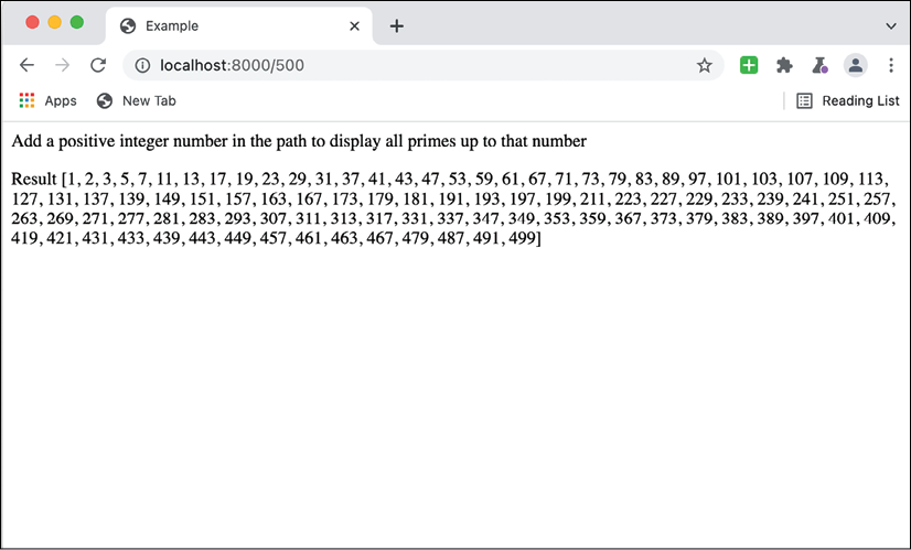
Figure 14.3: The interface displaying all primes up to 500

As you can see, we have an understandable output. Let's move on to profiling the process we used to get it.

Profiling the whole process

We can profile the whole process by starting it under cProfile and then capturing its output with. We start it like this, make a single request to http://localhost:8000/500, and check the results.

$ python3 -m cProfile -o server.prof server.py
Server available at http://localhost:8000
Use CTR+C to stop it
127.0.0.1 - - [10/Oct/2021 14:05:34] "GET /500 HTTP/1.1" 200 -
127.0.0.1 - - [10/Oct/2021 14:05:34] "GET /favicon.ico HTTP/1.1" 200 -
^CServer stopped.

We have stored the results in the file server.prof. This file can then be analyzed as before, using snakeviz.

$ snakeviz server.prof
snakeviz web server started on 127.0.0.1:8080; enter Ctrl-C to exit

Which displays the following diagram:

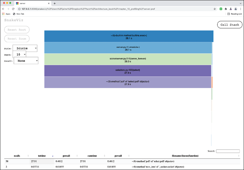
Figure 14.4: Diagram of the full profile. The full page is too big to fit here and has been cropped purposefully to show some of the info.

As you can see, the diagram shows that for the vast majority of the test duration, the code was waiting for a new request, and internally doing a poll action. This is part of the server code and not our code.

To find the code that we care about, we can manually search in the long list below for get_result, which is the root of the interesting bits of our code. Be sure to select Cutoff: None to display all the functions.

Once selected, the diagram will display from there onward. Be sure to scroll up to see the new diagram.

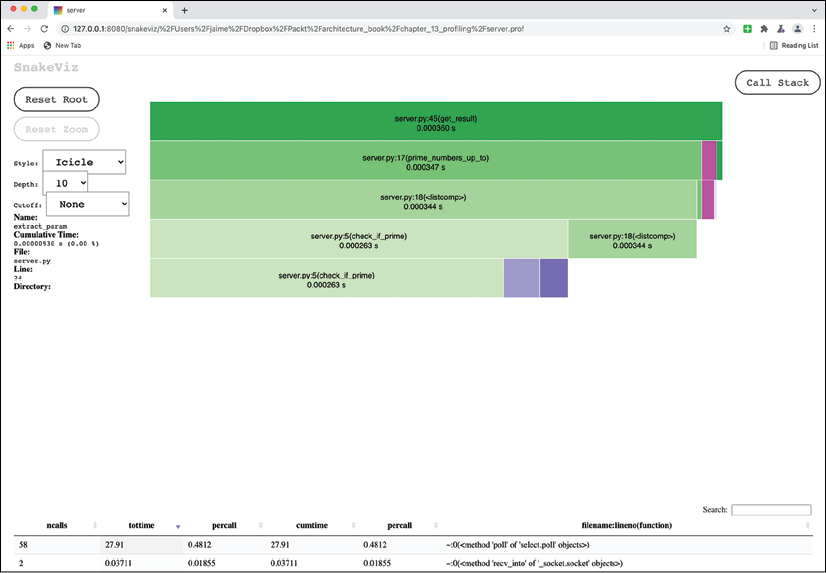
Figure 14.5: The diagram showing from get_result. The full page is too big to fit here and has been cropped purposefully to show some of the info.

Here, you can see more of the general structure of the code execution. You can see that most of the time is spent on the multiple check_if_prime calls, which comprise the bulk of prime_numbers_up_to and the list comprehension included in it, and very little time is spent on extract_params.

But this approach has some problems:

• First of all, we need to go a full cycle between starting and stopping a process. This is cumbersome to do for requests.
• Everything that happens in the cycle is included. That adds noise to the analysis. Fortunately, we knew that the interesting part was in get_result, but that may not be evident. This case also uses a minimal structure but adding that in the case of a complex framework like Django can lead to a lot of .
• If we process two different requests, they will be added into the same file, again mixing the results.

These problems can be solved by applying the profiler to only the part that is of interest and producing a new file for each request.

Generating a profile file per request

To be able to generate a different file with information per individual request, we need to create a decorator for easy access. This will profile and produce an independent file.

In the file server_profile_by_request.py, we get the same code as in server.py, but adding the following decorator.

from functools import wraps
import cProfile
from time import time
def profile_this(func):
    @wraps(func)
    def wrapper(*args, **kwargs):
        prof = cProfile.Profile()
        retval = prof.runcall(func, *args, **kwargs)
        filename = f'profile-{time()}.prof'
        prof.dump_stats(filename)
        return retval
    return wrapper

The decorator defines a wrapper function that replaces the original function. We use the wraps decorator to keep the original name and docstring.

Inside, we start a profiler and run the function under it using the runcall function. This line is the core of it – using the profiler generated, we run the original function func with its parameters and store its returned value.

retval = prof.runcall(func, *args, **kwargs)

After that, we generate a new file that includes the current time and dump the stats in it with the .dump_stats call.

We also decorate the get_result function, so we start our profiling there.

@profile_this
def get_result(path):
    param = extract_param(path)
    if param is None:
        return 'Invalid parameter, please add an integer'
    return prime_numbers_up_to(param)

The full code is available in the file server_profile_by_request.py, available on GitHub at https://github.com/PacktPublishing/Python-Architecture-Patterns/blob/main/chapter_14_profiling/server_profile_by_request.py.

Let's start the server now and make some calls through the browser, one to http://localhost:8000/500 and another to http://localhost:8000/800.

$ python3 server_profile_by_request.py
Server available at http://localhost:8000
Use CTR+C to stop it
127.0.0.1 - - [10/Oct/2021 17:09:57] "GET /500 HTTP/1.1" 200 -
127.0.0.1 - - [10/Oct/2021 17:10:00] "GET /800 HTTP/1.1" 200 -

We can see how new files are created:

$ ls profile-*
profile-1633882197.634005.prof 
profile-1633882200.226291.prof

These files can be displayed using snakeviz:

$ snakeviz profile-1633882197.634005.prof
snakeviz web server started on 127.0.0.1:8080; enter Ctrl-C to exit

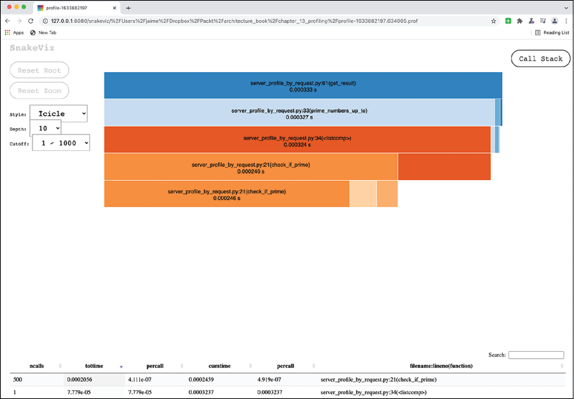
Figure 14.6: The profile information of a single request. The full page is too big to fit here and has been cropped purposefully to show some of the info.

Each file contains only the information from get_result onwards, which gets information only up to a point. Even more so, each file displays information only for a specific request, so it can be profiled individually, with a high level of detail.

The code can be adapted to adapt the filename more specifically to include details like call parameters, which can be useful. Another interesting possible adaptation is to create a random sample, so only 1 in X calls produces profiled code. This can help reduce the overhead of profiling and allow you to completely profile some requests.

Next, we'll see how to perform memory profiling.

Memory profiling

Sometimes, applications use too much memory. The worst-case scenario is that they use more and more memory as time goes by, normally due to what's called a memory leak, maintaining memory that is no longer used, due to some mistake in the coding. Other problems can also include the fact that the usage of memory may be improved, as it's a limited resource.

To profile memory and analyze what the objects are that use the memory, we need first to create some example code. We will generate enough Leonardo numbers.

Leonardo numbers are numbers that follow a sequence defined as the following:

• The first Leonardo number is one
• The second Leonardo number is also one
• Any other Leonardo number is the two previous Leonardo numbers plus one

Leonardo numbers are similar to Fibonacci numbers. They are actually related to them. We use them instead of Fibonacci to show more variety. Numbers are fun!

We present the first 35 Leonardo numbers by creating a recursive function and store it in leonardo_1.py, available on GitHub at https://github.com/PacktPublishing/Python-Architecture-Patterns/blob/main/chapter_14_profiling/leonardo_1.py.

def leonardo(number):
    if number in (0, 1):
        return 1
    return leonardo(number - 1) + leonardo(number - 2) + 1
NUMBER = 35
for i in range(NUMBER + 1):
    print('leonardo[{}] = {}'.format(i, leonardo(i)))

You can run the code and see it takes progressively longer.

$ time python3 leonardo_1.py
leonardo[0] = 1
leonardo[1] = 1
leonardo[2] = 3
leonardo[3] = 5
leonardo[4] = 9
leonardo[5] = 15
...
leonardo[30] = 2692537
leonardo[31] = 4356617
leonardo[32] = 7049155
leonardo[33] = 11405773
leonardo[34] = 18454929
leonardo[35] = 29860703
real      0m9.454s
user      0m8.844s
sys 0m0.183s

To speed up the process, we see that it's possible to use memorization techniques, which means to store the results and use them instead of calculating them all the time.

We change the code like this, creating the leonardo_2.py file (available on GitHub at https://github.com/PacktPublishing/Python-Architecture-Patterns/blob/main/chapter_14_profiling/leonardo_2.py).

CACHE = {}
def leonardo(number):
    if number in (0, 1):
        return 1
    if number not in CACHE:
        result = leonardo(number - 1) + leonardo(number - 2) + 1
        CACHE[number] = result
    return CACHE[number]
NUMBER = 35000
for i in range(NUMBER + 1):
    print(f'leonardo[{i}] = {leonardo(i)}')

This uses a global dictionary, CACHE, to store all Leonardo numbers, speeding up the process. Note that we increased the number of numbers to calculate from 35 to 35000, a thousand times more. The process runs quite quickly.

$ time python3 leonardo_2.py
leonardo[0] = 1
leonardo[1] = 1
leonardo[2] = 3
leonardo[3] = 5
leonardo[4] = 9
leonardo[5] = 15
...
leonardo[35000] = ...
real      0m15.973s
user      0m8.309s
sys       0m1.064s

Let's take a look now at memory usage.

Using memory_profiler

Now that we have our application storing information, let's use a profiler to show where the memory is stored.

We need to install the package memory_profiler. This package is similar to line_profiler.

$ pip install memory_profiler

We can now add a @profile decorator in the leonardo function (stored in leonardo_2p.py, on GitHub at https://github.com/PacktPublishing/Python-Architecture-Patterns/blob/main/chapter_14_profiling/leonardo_2p.py), and run it using the memory_profiler module. You'll notice that it runs slower this time, but after the usual result, it displays a table.

$ time python3 -m memory_profiler leonardo_2p.py
...
Filename: leonardo_2p.py
Line #    Mem usage    Increment  Occurences   Line Contents
============================================================
     5  104.277 MiB   97.082 MiB      104999   @profile
     6                                         def leonardo(number):
     7
     8  104.277 MiB    0.000 MiB      104999       if number in (0, 1):
     9   38.332 MiB    0.000 MiB           5           return 1
    10
    11  104.277 MiB    0.000 MiB      104994       if number not in CACHE:
    12  104.277 MiB    5.281 MiB       34999           result = leonardo(number - 1) + leonardo(number - 2) + 1
    13  104.277 MiB    1.914 MiB       34999           CACHE[number] = result
    14
    15  104.277 MiB    0.000 MiB      104994       return CACHE[number]
Real      0m47.725s
User      0m25.188s
sys 0m10.372s

This table shows first the memory usage, and the increment or decrement, as well as how many times each line appears.

You can see the following:

• Line 9 gets executed only a few times. When it does, the amount of memory is around 38 MiB, which will be the minimum memory used by the program.
• The total memory used is almost 105 MiB.
• The whole memory increase is localized in lines 12 and 13, when we create a new Leonardo number and when we store it in the CACHE dictionary. Note how we are never releasing memory here.

We don't really need to keep all the previous Leonardo numbers in memory at all times, and we can try a different approach to keep only a few.

Memory optimization

We create the file leonardo_3.py with the following code, available on GitHub at https://github.com/PacktPublishing/Python-Architecture-Patterns/blob/main/chapter_14_profiling/leonardo_3.py:

CACHE = {}
@profile
def leonardo(number):
    if number in (0, 1):
        return 1
    if number not in CACHE:
        result = leonardo(number - 1) + leonardo(number - 2) + 1
        CACHE[number] = result
    ret_value = CACHE[number]
    MAX_SIZE = 5
    while len(CACHE) > MAX_SIZE:
        # Maximum size allowed,
        # delete the first value, which will be the oldest
        key = list(CACHE.keys())[0]
        del CACHE[key]
    return ret_value
NUMBER = 35000
for i in range(NUMBER + 1):
    print(f'leonardo[{i}] = {leonardo(i)}')

Note we keep the @profile decorator to run the memory profiler again. Most of the code is the same, but we added the following extra block:

    MAX_SIZE = 5
    while len(CACHE) > MAX_SIZE:
        # Maximum size allowed,
        # delete the first value, which will be the oldest
        key = list(CACHE.keys())[0]
        del CACHE[key]

This code will keep the number of elements in the CACHE dictionary within a limit. When the limit is reached, it will remove the first element returned by CACHE.keys(), which will be the oldest.

The dictionary won't be able to grow. Let's now try to run it and see the results of the profiling.

$ time python3 -m memory_profiler leonardo_3.py
...
Filename: leonardo_3.py
Line #    Mem usage    Increment  Occurences   Line Contents
============================================================
     5   38.441 MiB   38.434 MiB      104999   @profile
     6                                         def leonardo(number):
     7
     8   38.441 MiB    0.000 MiB      104999       if number in (0, 1):
     9   38.367 MiB    0.000 MiB           5           return 1
    10
    11   38.441 MiB    0.000 MiB      104994       if number not in CACHE:
    12   38.441 MiB    0.008 MiB       34999           result = leonardo(number - 1) + leonardo(number - 2) + 1
    13   38.441 MiB    0.000 MiB       34999           CACHE[number] = result
    14
    15   38.441 MiB    0.000 MiB      104994       ret_value = CACHE[number]
    16
    17   38.441 MiB    0.000 MiB      104994       MAX_SIZE = 5
    18   38.441 MiB    0.000 MiB      139988       while len(CACHE) > MAX_SIZE:
    19                                                 # Maximum size allowed,
    20                                                 # delete the first value, which will be the oldest
    21   38.441 MiB    0.000 MiB       34994           key = list(CACHE.keys())[0]
    22   38.441 MiB    0.000 MiB       34994           del CACHE[key]
    23
    24   38.441 MiB    0.000 MiB      104994       return ret_value

In this case, we see how the memory remains stable at around the 38 MiB, that we see is the minimum. In this case, note how there are no increments or decrements. Really what happens here is that increments and decrements are too small to be noticed. Because they cancel each other, the report is close to zero.

The memory-profiler module is also able to perform more actions, including showing the usage of memory based on time and plotting it, so you can see memory increasing or decreasing over time. Take a look at its full documentation at https://pypi.org/project/memory-profiler/.

Summary

In this chapter, we described what profiling is and when it's useful to apply it. We described that profiling is a dynamic tool that allows you to understand how code runs. This information is useful in understanding the flow in a practice situation and being able to optimize the code with that information. Code can be optimized normally to execute faster, but other alternatives are open, like using fewer resources (normally memory), reducing external accesses, etc.

We described the main types of profilers: deterministic profilers, statistical profilers, and memory profilers. The first two are mostly oriented toward improving the performance of code and memory profilers analyze the memory used by the code in execution. Deterministic profilers instrument the code to detail the flow of the code as it's executed. Statistical profilers sample the code at periodic times to provide a general view of the parts of the code that are executed more often.

We then showed how to profile the code using deterministic profilers, presenting an example. We analyzed it first with the built-in module cProfile, which gives a function resolution. We saw how to use graphical tools to show the results. To dig deeper, we used the third-party module line-profiler, which goes through each of the code lines. Once the flow of the code is understood, it is optimized to greatly reduce its execution time.

The next step was to see how to profile a process intended to keep running, like a web server. We showed the problems with trying to profile the whole application in these cases and described how we can profile each individual request instead for clarity.

Finally, we also presented an example to profile memory and see how it's used by using the module memory-profiler.

In the next chapter, we will learn more details about how to find and fix problems in code, including in complex situations, through debugging techniques.

Join our book’s Discord space

Join the book’s Discord workspace for a monthly Ask me Anything session with the authors:

https://packt.link/PythonArchitechture