Scenario 5 - solving linearly non-separable problems

The hyperplane we have looked at till now is linear, for example, a line in a two-dimensional feature space, a surface in a three-dimensional one. However, in frequently seen scenarios like the following one, we are not able to find any linear hyperplane to separate two classes.

Intuitively, we observe that data points from one class are closer to the origin than those from another class. The distance to the origin provides distinguishable information. So we add a new feature and transform the original two-dimensional space into a three-dimensional one. In the new space, we can find a surface hyperplane separating the data, or a line in the 2D view. With the additional feature, the dataset becomes linearly separable in the higher dimensional space .

Similarly, SVM with kernel solves nonlinear classification problems by converting the original feature space to a higher dimensional feature space with a transformation function such that the transformed dataset is linearly separable. A linear hyperplane is then trained based on observations . For an unknown sample , it is first transformed into ; the predicted class is determined by .

Besides enabling nonlinear separation, SVM with kernel makes the computation efficient. There is no need to explicitly perform expensive computation in the transformed high-dimensional space. This is because:

During the course of solving the SVM quadratic optimization problems, feature vectors are only involved in the final form of pairwise dot product , although we did not expand this mathematically in previous sections. With kernel, the new feature vectors are and their pairwise dot products can be expressed as follows:

Where the low dimensional pairwise dot product can be first implicitly computed and later mapped to a higher dimensional space by directly applying the transformation function. There exists a functions K that satisfies the following:

Where function K is the so-called kernel function. As a result, the nonlinear decision boundary can be efficiently learned by simply replacing the terms  with .

The most popular kernel function is the radial basis function (RBF) kernel (also called Gaussian kernel), which is defined as follows:

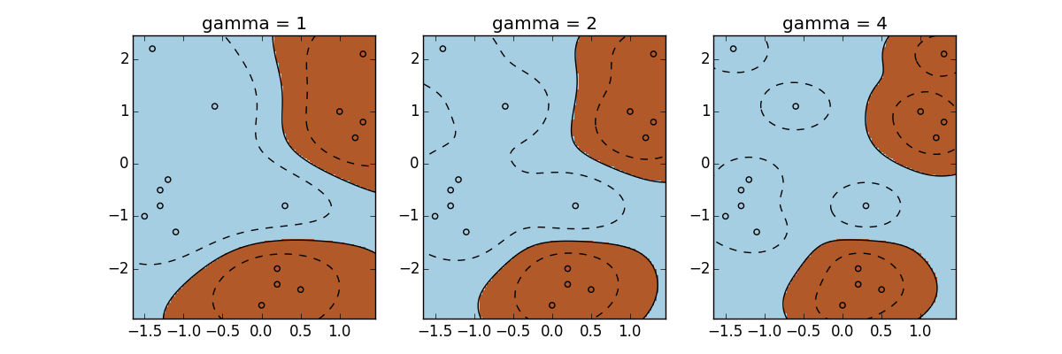
Where . In the Gaussian function, the standard deviation controls the amount of variation or dispersion allowed-the higher (or lower ), the larger width of the bell, the wider range of values that the data points are allowed to spread out over. Therefore, as the kernel coefficient determines how particularly or generally the kernel function fits the observations. A large indicates a small variance allowed and a relatively exact fit on the training samples, which leads to a high bias. On the other hand, a small implies a high variance and a generalized fit, which might cause overfitting. To illustrate this, let's apply RBF kernel with different values to a dataset:

>>> import numpy as np
>>> import matplotlib.pyplot as plt
>>> X = np.c_[# negative class
...           (.3, -.8),
...           (-1.5, -1),
...           (-1.3, -.8),
...           (-1.1, -1.3),
...           (-1.2, -.3),
...           (-1.3, -.5),
...           (-.6, 1.1),
...           (-1.4, 2.2),
...           (1, 1),
...           # positive class
...           (1.3, .8),
...           (1.2, .5),
...           (.2, -2),
...           (.5, -2.4),
...           (.2, -2.3),
...           (0, -2.7),
...           (1.3, 2.1)].T
>>> Y = [-1] * 8 + [1] * 8
>>> gamma_option = [1, 2, 4] 

We will visualize the dataset with corresponding decision boundary trained under each of the preceding three :

>>> import matplotlib.pyplot as plt
>>> plt.figure(1, figsize=(4*len(gamma_option), 4))
>>> for i, gamma in enumerate(gamma_option, 1):
...     svm = SVC(kernel='rbf', gamma=gamma)
...     svm.fit(X, Y)
...     plt.subplot(1, len(gamma_option), i)
...     plt.scatter(X[:, 0], X[:, 1], c=Y, zorder=10, 
                                          cmap=plt.cm.Paired)
...     plt.axis('tight')
...     XX, YY = np.mgrid[-3:3:200j, -3:3:200j]
...     Z = svm.decision_function(np.c_[XX.ravel(), YY.ravel()])
...     Z = Z.reshape(XX.shape)
...     plt.pcolormesh(XX, YY, Z > 0, cmap=plt.cm.Paired)
...     plt.contour(XX, YY, Z, colors=['k', 'k', 'k'],   
                linestyles=['--', '-', '--'], levels=[-.5, 0, .5])
...     plt.title('gamma = %d' % gamma)
>>> plt.show()

Again, can be fine-tuned via cross-validation to obtain the best performance.

Some other common kernel functions include the polynomial kernel and sigmoid kernel:

In the absence of expert prior knowledge of the distribution, RBF is usually preferable in practical use, as there are more parameters (the polynomial degree d) to tweak for the Polynomial kernel and the empirically sigmoid kernel can perform approximately on par with RBF only under certain parameters. Hence it is mainly a debate between the linear and RBF kernel.