Now the question is how we can obtain the optimal w such that is minimized. We do so via gradient descent.

Gradient descent (also called steepest descent) is a procedure of minimizing an objective function by first-order iterative optimization. In each iteration, it moves a step that is proportional to the negative derivative of the objective function at the current point. This means the to-be-optimal point iteratively moves downhill towards the minimal value of the objective function. The proportion we just mentioned is called learning rate, or step size. It can be summarized in a mathematical equation:

Where the left w is the weight vector after a learning step, and the right w is the one before moving, is the learning rate and is the first-order derivative, the gradient.

In our case, let's start with the derivative of the cost function with respect to w. It might require some knowledge of calculus, but no worries; we will walk through it step by step.

We first calculate the derivative of with respect to w. We herein take the j-th weight w_j as an example (note , and we omit the ⁽ⁱ⁾ for simplicity):

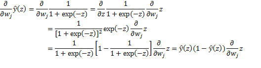
Then the derivative of the sample cost J(w):

And finally the entire cost over m samples:

Generalize it to :

Combined with the preceding derivations, the weights can be updated as follows:

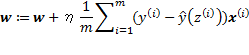
w gets updated in each iteration. After a substantial number of iterations, the learned w and b are then used to classify a new sample as follows:

The decision threshold is 0.5 by default, but it definitely can be other values. In a case where the false negative is by all means supposed to be avoided, for example predicting fire occurrence (positive class) for alert, the decision threshold can be lower than 0.5, such as 0.3, depending on how paranoid we are and how proactively we want to prevent the positive event from happening. On the other hand, when the false positive class is the one that should be evaded, for instance predicting product success (positive class) rate for quality assurance, the decision threshold can be greater than 0.5, such as 0.7, based on how high the standard we set is.

With a thorough understanding of the gradient descent-based training and predicting process, we now implement the logistic regression algorithm from scratch.

We start with defining the function computing the prediction  with current weights:

>>> def compute_prediction(X, weights):
...     """ Compute the prediction y_hat based on current weights
...     Args:
...         X (numpy.ndarray)
...         weights (numpy.ndarray)
...     Returns:
...         numpy.ndarray, y_hat of X under weights
...     """
...     z = np.dot(X, weights)
...     predictions = sigmoid(z)
...     return predictions  

With this, we are able to continue with the function updating the weights by one step in a gradient descent manner:

>>> def update_weights_gd(X_train, y_train, weights,
                                            learning_rate):
...     """ Update weights by one step
...     Args:
...         X_train, y_train (numpy.ndarray, training data set)
...         weights (numpy.ndarray)
...         learning_rate (float)
...     Returns:
...         numpy.ndarray, updated weights
...     """
...     predictions = compute_prediction(X_train, weights)
...     weights_delta = np.dot(X_train.T, y_train - predictions)
...     m = y_train.shape[0]
...     weights += learning_rate / float(m) * weights_delta
...     return weights  

And the function calculating the cost J(w) as well:

>>> def compute_cost(X, y, weights):
...     """ Compute the cost J(w)
...     Args:
...         X, y (numpy.ndarray, data set)
...         weights (numpy.ndarray)
...     Returns:
...         float
...     """
...     predictions = compute_prediction(X, weights)
...     cost = np.mean(-y * np.log(predictions) 
                       - (1 - y) * np.log(1 - predictions))
...     return cost  

Now we connect all these functions together with the model training function by:

• Updating the weights vector in each iteration
• Printing out the current cost for every 100 (can be other values) iterations to ensure that cost is decreasing and things are on the right track

>>> def train_logistic_regression(X_train, y_train, max_iter, 
                           learning_rate, fit_intercept=False):
...     """ Train a logistic regression model
...     Args:
...         X_train, y_train (numpy.ndarray, training data set)
...         max_iter (int, number of iterations)
...         learning_rate (float)
...         fit_intercept (bool, with an intercept w0 or not)
...     Returns:
...         numpy.ndarray, learned weights
...     """
...     if fit_intercept:
...         intercept = np.ones((X_train.shape[0], 1))
...         X_train = np.hstack((intercept, X_train))
...     weights = np.zeros(X_train.shape[1])
...     for iteration in range(max_iter):
...         weights = update_weights_gd(X_train, y_train, 
                                        weights, learning_rate)
...         # Check the cost for every 100 (for example)       
              iterations
...         if iteration % 100 == 0:
...             print(compute_cost(X_train, y_train, weights))
...     return weights  

And finally, predict the results of new inputs using the trained model:

>>> def predict(X, weights):
...     if X.shape[1] == weights.shape[0] - 1:
...         intercept = np.ones((X.shape[0], 1))
...         X = np.hstack((intercept, X))
...     return compute_prediction(X, weights)  

Implementing logistic regression is very simple as we just saw. Let's examine it with a small example:

>>> X_train = np.array([[6, 7],
...                     [2, 4],
...                     [3, 6],
...                     [4, 7],
...                     [1, 6],
...                     [5, 2],
...                     [2, 0],
...                     [6, 3],
...                     [4, 1],
...                     [7, 2]])
>>> y_train = np.array([0,
...                     0,
...                     0,
...                     0,
...                     0,
...                     1,
...                     1,
...                     1,
...                     1,
...                     1])  

Train a logistic regression model by 1000 iterations, at learning rate 0.1 based on intercept-included weights:

>>> weights = train_logistic_regression(X_train, y_train, 
             max_iter=1000, learning_rate=0.1, fit_intercept=True)
0.574404237166
0.0344602233925
0.0182655727085
0.012493458388
0.00951532913855
0.00769338806065
0.00646209433351
0.00557351184683
0.00490163225453
0.00437556774067  

The decreasing cost means the model is being optimized. We can check the model's performance on new samples:

>>> X_test = np.array([[6, 1],
...                    [1, 3],
...                    [3, 1],
...                    [4, 5]])
>>> predictions = predict(X_test, weights)
>>> predictions
array([ 0.9999478 ,  0.00743991,  0.9808652 ,  0.02080847])  

To visualize it, use the following:

>>> plt.scatter(X_train[:,0], X_train[:,1], c=['b']*5+['k']*5, 
                                                      marker='o')  

Use 0.5 as the classification decision threshold:

>>> colours = ['k' if prediction >= 0.5 else 'b' 
                                  for prediction in predictions]
>>> plt.scatter(X_test[:,0], X_test[:,1], marker='*', c=colours)
>>> plt.xlabel('x1')
>>> plt.ylabel('x2')
>>> plt.show()  

The model we trained correctly predicts new samples (the preceding stars).