

chapter 9
The Harmonic Oscillator
One of the most important concepts in physics is the harmonic oscillator. In this chapter we will explore the behavior of a harmonic oscillator in quantum mechanics.
CHAPTER OBJECTIVES
In this chapter you will
• learn the hamiltonian for the harmonic oscillator
• calculate the eigenstates and energies of the harmonic oscillator
• learn about the raising and lowering or ladder operators
The harmonic oscillator for a particle of mass m is described by the potential V = 1/2kx2 where k = mω2. Solutions to the Schrödinger equation for this potential are given in terms of Hermite polynomials, and they can be obtained by either working in the position representation or using an algebraic method based on the raising and lowering operators.
The Solution of the Harmonic Oscillator in the Position Representation
The Hamiltonian for the harmonic oscillator in one dimension is
where ω is the angular frequency and m is the mass of the oscillator. The time-independent Schrödinger equation takes the form
Typically, dimensionless parameters are introduced for the position coordinate and the energy
The Schrödinger equation can then be rewritten as
where ψ = ψ(u). Solutions to this equation can be obtained by using the series method; we simply summarize them here. They are a product of an exponential and a Hermite polynomial
In terms of the position coordinate, the solution takes the form

Here An is a normalization constant. Figures 9-1, 9-2, and 9-3 show the form of the first three wavefunctions.
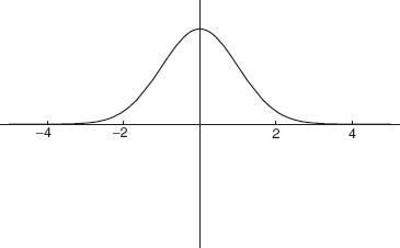
FIGURE 9-1

FIGURE 9-2

FIGURE 9-3
Show that the ground state wavefunction of the harmonic oscillator
is normalized. If a harmonic oscillator is in this state, find the probability that the particle can be found in the range 0 ≤ x ≤ 1.
To check normalization, we begin by squaring the wavefunction
Recalling that
we now set z2 = (mω/ ) x2. Then we have
We invert this relation to give
Using these substitutions, the normalization integral becomes

Therefore the state is normalized. The probability that the particle is found in the range 0 ≤ x ≤ 1 is given by
This integral is nearly in the form of the error function
Following the procedure used in checking normalization, we set
and obtain

DEFINITION: Normalization of the Hermite Polynomials
The normalization of the wavefunctions comes from that of the Hermite polynomials. The orthonormality of the Hermite polynomials is written as
Using this relationship, we can normalize the wavefunctions by integrating with the normalization constant

To have a normalized wavefunction, this must be equal to unity, and so we have

We can then write the normalized wavefunction as

The energy is found from the series solution technique applied to the Schrödinger equation. The termination condition for this solution dictates that the energy of state n is given by
Helpful recursion relationships exist that can be used to derive higher-order Hermite polynomials. These include

The first few Hermite polynomials are given by

The recursion relations can be useful for determining expectation values.
Find H4 (u).
Using the recursion formula
and setting n + 1= 4, we obtain

Show that
is an eigenfunction of the dimensionless equation
and find the corresponding eigenvalue. Use the relationships used to derive the dimensionless parameters to find the energy that this represents for a particle in the harmonic oscillator potential. Find the energy level.

We rewrite the dimensionless equation by moving the energy term to the other side:
Using the result obtained for the second derivative, the left-hand side is
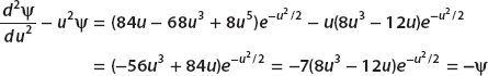
and so we have
Now we recall that
Solving for E, we obtain
To determine the energy level, we recall that the energy of the harmonic oscillator is
So we rewrite the expression we have derived in this form:
Therefore we see that this is the n = 3 excited state of the harmonic oscillator.
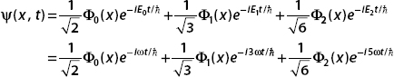
Suppose that a particle is in the state
Write down the state at time t and show that it oscillates in time.
If the initial wavefunction is in some superposition of basis states
then by setting E = ω, the time evolution of the state can be written as
We apply this procedure to the wavefunction as stated in the problem

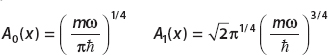
Now we turn to the problem of finding the expectation value. The exact form of the basis states is

For simplicity we denote
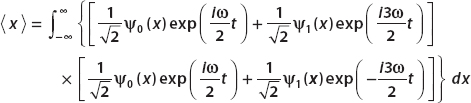
We will also use the frequently seen integrals

So the expectation value of position for the given state is
First, we simplify the integrand

and so we obtain

The first two terms vanish because 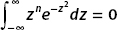 . To see this, recall that
and perform a substitution. The second integral vanishes for the same reason. Therefore we are left with

This can be rewritten as

But
and so we find that the expectation value is
We see that the expectation value oscillates in time with frequency ω.
The Operator Method for the Harmonic Oscillator
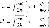
We now proceed to solve the harmonic oscillator problem, using an entirely different method based on operators and algebra alone. Consider the following operators defined in terms of the position and momentum operators:
We can rewrite the Hamiltonian, using these operators, and then solve the eigenvector/eigenvalue problem in an algebraic way. An important part of working with these operators is to determine their commutator.
Derive the commutator [a, a†].
To find this commutator, we rely on [x, p] = i:
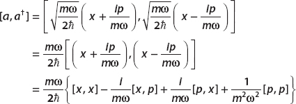
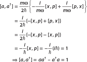
Since [x, x] = [p, p] = 0, this simplifies to
Show that the harmonic oscillator Hamiltonian can be written in the form
We begin by writing the position and momentum operators in terms of a and a†. Notice that
and so the position operator can be written as
The harmonic oscillator Hamiltonian contains the square of x. Squaring this term, we find
Now we write the momentum operator in terms of a and a†. Consider

And so we can write momentum as
Now we can insert these terms into the Hamiltonian
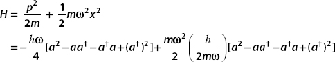
Notice that
Therefore the a2 and (a†)2 terms cancel. This leaves
Now we use the commutation relation [a, a†] = aa† − a†a = 1 to write aa† = 1 + a†a, and we have
Some other important commutation relations are
Number States of the Harmonic Oscillator
Now that we have expressed the Hamiltonian in terms of the operators a and a†, we can derive the energy eigenstates. We begin by stating the eigenvalue equation
To simplify notation, we set  . We have already seen that
Using the form of the Hamiltonian written in terms of a and a†, we find that
However, we know that
Equating this to the above, we have
Now divide through by ω and subtract the common term  from both sides, giving
This shows that the energy eigenstate is an eigenstate of a†a with eigenvalue n. The operator a†a is called the number operator.
SUMMARY
The number operator N is defined in the following way:
The state |n_ is sometimes referred to as the number state. the lowest possible state for the harmonic oscillator is the state  , and it is called the ground state.
Energy levels of the harmonic oscillator are equally spaced, and we move up and down the ladder of energy states, using the operators a and a†.
Using [H, a] = −ωa and [H, a†] = − ωa†, show that
  is an eigenvector of H with eigenvalue En − ω and that
  is an eigenvector of H with eigenvalue En + ω.
First we write the commutator explicitly:
Now we apply this to state :
On the first term, we use
giving
From this we see that a steps the energy down by ω. Because of this, this operator is called the lowering operator. We now follow the same procedure for . Beginning with the commutator
we obtain

From this we see that a† steps up the energy by one unit of ω. This gives it its name, the raising operator. Together these operators are sometimes known as ladder operators.
At time t = 0, a wavefunction is in the state
(a) If the energy is measured, what values can be found and with what probabilities?
(b) Find the average value of the energy  .
.
(c) Find the explicit forms of Φi(x), the basis functions for this expansion, and write the form of the wavefunction at time t.
(a) Using the energy of the nth eigenstate En = (n + 1/2)ω, we make a table of possible energies for the basis states found in this wave-function (Table 9-1).

Notice that these probabilities sum to 1:
(b) The average energy is found to be

(c) The nth state wavefunction of the harmonic oscillator is
Therefore we have

At time t, the wavefunction is given by
More on the Action of the Raising and Lowering Operators
We now work out the action of the raising and lowering operators on the eigenstates of the Hamiltonian. We begin by applying the commutator [H a†] to an arbitrary number state
On the left-hand side we expand the commutator

Now we equate this to 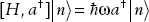
We move terms over to the right side and combine, giving
From this we conclude that is an eigenvector of H with eigenvalue ω(n + 3/2). Now if
Therefore we conclude that
The operator a† raises the state  to
to  (this is why it is called the raising operator). A similar exercise shows that
Since the lowest state of the harmonic oscillator is the ground state, we cannot lower below  . To avoid going lower than this state, the lowering operator annihilates the state
The nth eigenstate can be obtained from the ground state by application of a†n times to the ground state
Summary
In this chapter we learned how to handle the harmonic oscillator in quantum mechanics and how to write the Hamiltonian in terms of the ladder operators.
QUIZ
1. A harmonic oscillator is in the state
A. Find A so that the state is normalized.
B. A measurement is made of the energy. What energies can be found? What is the probability of obtaining each value of the energy?
C. Find the state of the system at a later time t.
2. Show that the harmonic oscillator Hamiltonian can be written as
3. Use H = ω(aa† − 1/2) to show that  .
.
4. Use the fact that  to explain why a = 0.
5. Show that
6. Use the recursion relations for the Hermite polynomials to find  and
and  for the ground state of the harmonic oscillator in the coordinate representation.
..................Content has been hidden....................
You can't read the all page of ebook, please click here login for view all page.