

chapter 16
Time-Dependent Perturbation Theory
Many Hamiltonians which describe real systems have a time-dependent part. In this case, we need to extend the techniques of perturbation theory.
CHAPTER OBJECTIVES
In this chapter you will
• Learn how to handle a time-dependent hamiltonian
• Find the probability of a system changing state with a time-dependent hamiltonian
• Learn the different pictures in quantum theory
Now consider a Hamiltonian that can be written in terms of a time-independent part which we dub H0 and a time-dependent potential V:
If the time-dependent piece V is small compared to the time-independent piece H0, we can use perturbation theory to solve a problem involving this type of Hamiltonian. When we apply time-independent perturbation theory, the goal was to correct energy levels. In this case, however, we will not correct energies, but will instead be looking at transitions between states. In particular, we wish to find the probabilities of transition between states occurring.
Generally speaking, we start with a known piece, which are the solutions to the time-independent part of the problem. That is we know the eigenstates and energies of H0:
The problem in time-dependent perturbation theory, then, is that given the system in state
with energy
Em
we wish to find the probability that at a later time the system is in the state
with energy
En
Now let’s start with a zero time-dependent potential
Then the wavefunction has the expansion in terms of energy eigenstates:
where |cn|2 is the probability that the system is in state  and normalization requires that
Now we introduce a time-dependent potential, and the coefficients become time-dependent, i.e.,

The task then becomes as stated above, to solve for the coefficients so that we can find the probability of transitions between states. To do this, we start in the usual way, by solving the time-dependent Schrödinger equation:
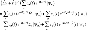
Expanding the state, we get
Let’s work out the left-hand side first:
Taking the inner product with
and using
we obtain

Now let’s tackle the right-hand side and equate the results. First we get
Now take the inner product with another state:

Setting the left and right sides equal gives us a differential equation that can be used to solve for the coefficients. First set both sides equal:
Now cancel this term from both sides:
and we are left with
Now let’s move the exponential on the left over to the other side:

Then we define the transition frequency
and we are left with
The terms involving the potential are matrix elements:
And so we can write this as a matrix differential equation:

The problem at hand is then to start with the system in an initial state at time t = 0:
and then determine the probability it is in some final state at time t :
The answer is found by solving for the probability amplitude cf (t). Using perturbation theory, in an analogous way to the time-independent case, we can find the answer to different orders. The first-order result is
The first-order approximation gives a good answer when the probability of transition between the states is small.
Consider a particle trapped in a one-dimensional infinite square well of width a. Suppose that the particle is subject to a perturbation of the form
If the particle is initially in the ground state, find the probability that at a later time t the particle is found in the first excited state. The particle states for the one-dimensional square well are shown in Figure 16-1.

FIGURE 16-1 • The states of a particle in an infinite square well. Given a time-dependent perturbation, we calculate the probability for a system initially in the ground state to be found later in the n = 2 excited state. Image created by Papa November.
To do the calculation, we will need the wavefunctions and energies of the unperturbed states. Recall that the wavefunctions are given by
with associated energy
The probability that the particle will be found in the first excited state can be approximately calculated using the expression
In this example,
So we need to calculate

Let’s do the time component first, which is straightforward enough:
As t′ → ∞,
is oscillatory, but it’s multiplied by
e−t′
which goes to zero. So the term at the upper limit is zero. Evaluated at the lower limit:
At the end we’re going to need the modulus of this squared, which is
We’ve ignored the minus sign from integration since it cancels when we calculated the term that’s going to contribute to the probability, which is the modulus squared.
Turning to the spatial part of the calculation, using the relevant wavefunctions, we have
According to Wolfram Alpha, this is

And so the probability for a transition between the ground state and the first excited state is
Now we have
So
“Pictures” in Quantum Theory
There are a few different ways to look at the time dependence of a system in quantum theory. The first one has been used throughout most of the book, namely, the Schrödinger picture. This can be summarized as follows:
• State vectors depend explicitly on time.
• Operators do not depend explicitly on time.
Since operators are in this case time-independent, this indicates the Schrödinger picture is most appropriate when dealing with a time-independent Hamiltonian. The central tenet, if you will, of the Schrödinger picture is of course that the Schrödinger equation is used to find the time evolution of the states:
The general solution as discussed above is
where the probability coefficients cn are time-independent.
An alternative machinery to which we briefly alluded in Chap. 8 is called the Heisenberg picture. This approach is characterized by the opposite extreme, namely,
• State vectors are not time-dependent.
• Operators are time-dependent.
A state vector in the Heisenberg picture is simply the state vector Schrödinger picture at the initial time, with the time evolution operator attached
In other words, at all time t it’s just the initial state vector. Operators, however, are obtained from Schrödinger operators by using the unitary time evolution operator on the left and the right to construct a time-dependent Heisenberg operator:
Operators in this picture satisfy the Heisenberg equation of motion:
We now turn to an alternative view which is more useful for time-dependent perturbation theory. It’s called the interaction picture, and it’s an intermediate between the two pictures we’ve seen so far. In this picture
• State vectors change with time.
• Operators change with time.
So state vectors and operators are time-dependent in the interaction picture. We begin by splitting the Hamiltonian into two parts, a time-independent piece and a time-dependent potential, just as described in the introductory section of this chapter:
A state in the interaction picture is then obtained from a Schrödinger state by using
Time evolution of the states is governed by a Schrödinger-type equation, but instead of the overall Hamiltonian we include only the time-dependent potential:
Operators in the interaction picture are time-dependent and satisfy the Heisenberg equation of motion; however, we include only the time-independent part of the Hamiltonian:
Two-Level Systems
In many practical applications, a system can be treated as having two energy levels, since the other states are basically inaccessible. In the old world we came from without a time-dependent Hamiltonian, we would have this for a two-level system—two states, two energy levels, and two probability coefficients that were time-independent:
Now with the time-dependent Hamiltonian, we need to put time dependence in the probability coefficients:
Given some time-dependent potential V, in most cases (but not all) the diagonal terms vanish, so we have a coupled set of differential equations for the coefficients:

Now let’s solve, using perturbation theory. We start with the initial conditions. Suppose that the system is in the ground state. This means that the coefficients are
c1(t) = 1 c2(t) = 0
This is the zero-order solution. To get the first-order solution, we use these values in the matrix equations:
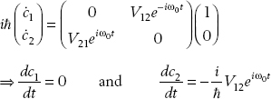
This implies that

This is the first-order solution. Putting these values in the matrix equation on the right-hand side, we obtain the second-order solution:

A two-level system is perturbed by a constant potential V =1 for t > 0. At t = 0, the system is in the ground state. Using first-order perturbation theory, find the probability of finding the system in the first excited state at some later time t.
Using

if the perturbation is constant, the matrix element can be taken outside of the integral:
Now

Let’s get the squared amplitude of this expression:

Therefore the probability of finding the system in the excited state at some later time is
This produces a transition probability which oscillates in time, as shown in Fig. 16-2. In Fig. 16-3, we see the probability amplitude in frequency space which shows an interference pattern. The peak is centered about the origin, showing that the system has a substantial probability to be found in the excited state only if the two states are close together in energy.
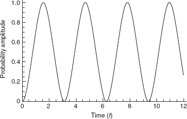
FIGURE 16-2 • A representation of the probability amplitude calculated in Example 16-2.

FIGURE 16-3 • The probability amplitude in frequency space.
Fermi’s Golden Rule
Consider a system perturbed by a harmonic potential of the form
If the system is in the initial state  , Fermi’s golden rule states that the probability transition rate for finding the system in the state
  is
is
The Emission and Absorption of Radiation
Now let’s consider an atom interacting with light, which means that the electron finds itself in the presence of an external, perturbing electromagnetic field. In general, the Hamiltonian is this ugly expression:
Here going from left to right, we’ve got momentum, the magnetic vector potential, the potential the electron normally finds itself in, the scalar electric potential, and spin dotted with the magnetic field. We could monkey around with this, but that horror is probably better suited for a more advanced treatment. Instead let’s consider the simplest case possible. For simplicity we’ll treat the radiation field classically and consider an electromagnetic wave polarized along the z axis:
This leads us to a perturbing Hamiltonian of the form
We’re going to kind of fudge. Although we’re describing a classical electromagnetic field, we’re going to imagine that atoms can absorb or emit photons of light, with each photon having energy
ε =  ω
ω
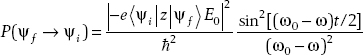
I used epsilon here just to avoid confusion with the electric field E. Now, in the Quiz, you will show that the transition probability for a system exposed to a harmonic perturbation assumes the form

We’re going to use this result in this case, almost exactly. An atom can transition to the final excited state if it absorbs a photon of energy ω. The probability for it to transition to the final excited state from the initial state is

This is the absorption process, but stimulated emission can also occur. In this case, the atom starts out in the excited state. Then you “stimulate” it by exposing it to some light. In our case, we direct a monochromatic wave polarized in the z direction at the atom. It then emits a photon of energy ω and drops down to the ground state. The transition probability for stimulated emission turns out to be the same as the probability for absorption:
The only difference is that the states have been swapped about, because we’re going from the excited state down to the ground state.
Now, an atom in the excited state can emit radiation even in the absence of an external electromagnetic field. This process is called spontaneous emission since there is no external agent (i.e., electromagnetic field) that would stimulate the emission. The transition rate in this case is given by the Einstein A coefficient:
Summary
In this chapter we learned about incorporating the case of a Hamiltonian with a time-dependent piece and illustrated calculations with a two-level system.
QUIZ
1. At t = −∞, a harmonic oscillator is in the ground state. At time t = 0, the system is exposed to a perturbation
Show that the probability for the system to be in the first excited state at t = +∞ is given by
2. Consider a particle trapped in a one-dimensional infinite square well of width a that is subjected to the perturbation
Show that the probability at a later time of finding it in the first excited state is
3. A two-level system is perturbed by a potential such that
If the system starts in the ground state, show that the probability of finding it in the excited state is proportional to
where ω0 = ω2 – ω1.
..................Content has been hidden....................
You can't read the all page of ebook, please click here login for view all page.