

Answers to Quiz and Exam Questions
Chapter 1
1. Given that
We see that
Some manipulation of the series given for g can put it in this form. We have
Using the geometric series result, we can write
Computing the derivative of f using this representation we find
So we can write g in the following way
2. The lowest energy of the hydrogen atom is
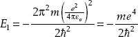
Now explicitly including the permittivity of free space, we have
Let’s take a look at the units, to see what value we should use for Planck’s constant. Since we want the final answer in electron volts, for the electron mass we use
where we included the speed of light in m/s. The units of εo are C2/N m2, and so using the fact that a Joule is a N-m we get the right units if we use the value of Planck’s constant written in terms of J-s. Writing charge in Coulombs (C) we would have

So, in addition to the mass of the electron defined above we use the following values
And we obtain

3. Use 
Chapter 2
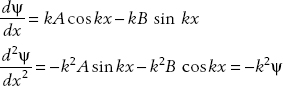
1. (a) Setting ψ(x, t) = ϕ(x) f(t) and using the Schrödinger equation, we have
For the right-hand side we obtain
Setting this equal to the time derivative and dividing through by ψ(x, t) = ϕ(x) f(t) gives
We have set these terms equal to a constant because on one side we have a function of t only while on the other side we have a function of x only, and the only possible way they can be equal is if they are each constant. We call the constant E in anticipation that this is the energy. Looking at the equation involving time we have
This integrates immediately to give
(b) For the given wavefunction we have
The result follows.
2. The complex conjugate of the wavefunction is
(a) 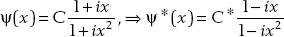
And so we find that
(b) To find the normalization constant we need to solve
It turns out that
And so 
(c) Using the following integral

we find that the probability is ≈0.52.
3. (a) The complex conjugate is
Therefore the normalization condition is
(b) The probability is given by
4. The expectation value is
This is an odd function, as we can see by looking at the plot

FIGURE 1
Therefore the integral vanishes. Now for  , we encounter the integral
Using L’Hopital’s rule, the first term goes to zero at the limits of integration, for example
For the second term, note that
So you should find that the expectation value is
5. The function given is not square integrable, so it cannot be a valid wavefunction. So, the question makes no sense.
6. X is Hermitian but i X is not.
7. You should find that 
8. Recall that for the infinite square well
(a)
Notice that
So the wavefunction can be rewritten as
Normalization requires that  where the cn are the coefficients of the expansion. In this case we have

Hence the wavefunction is normalized.
(b) The possible values of the energy are
(c)  . To see this consider that integrals such as
9. A wavefunction must be normalized, which means that the norm of the wavefunction must be 1, which is the same (mathematically) as a unit vector.
10. 
11. Probabilities cannot be negative.
12. The energies of bound states are quantized in quantum mechanics.
Chapter 3
1. B
2. A
3. B
4. C
5. A
6. B
7. A
8. C
Chapter 4
1. The inner products are
(A, B) = (2)(1) + (−4i)(0) + (0)(1) + (1)(9i) + (7i)(2) = 2 + 23i
(B, A) = (1)(2) + (0)(4i) + (1)(0) + (−9i)(1) + (2)(−7i) = 2 − 23i
2. To see if the functions belong to L2 we compute  and see if it is finite.
(a) In the first case we obtain
Since it is finite, the function belongs to L2.
(b) This integral diverges, so it does not belong to L2.
(c) In the final case we find
So the function belongs to L2.
3. By the sampling property of the delta function
Therefore if we write δ(x) then we set a to zero and
x δ(x) = (0)δ(x) = 0
(a) Do a u substitution in the integral
4. 0
5. 16
Chapter 5
1. (a) The inner products are
And so the norms are 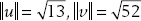 . The vectors are not normalized.
(b) 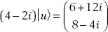
(c) 
2. The set of 2 × 2 matrices does constitute a vector space. For a basis, try the Pauli matrices and the identity matrix.
3. They are linearly independent.
4. No they are not, since we can write the third as a linear combination of the first two
5. We square the term on the left to obtain

Take the square root of both sides and the result follows.
6. The basis is
7. (a) The inner products are
And so the normalized vectors are
(b) The sum of the vectors is
(c)
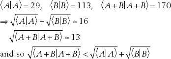
(d)

8. The dual vector is
(a) 
(b) The column vector representation is

(c) The row vector representation is
(d)  , to normalize divide by the square root of this quantity.
9. B
10. C
Chapter 6
1. The eigenvalues of all three matrices are ±1. The eigenvectors are

The matrices are Hermitian and unitary.
2. To do the proof, recall that A† = −A for an anti-Hermitian operator. Then we have
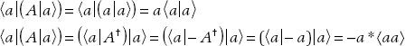
Comparison of the two equations shows that a = −a*, so a must be pure imaginary.
3. Assume that we have two eigenvectors of an operator A such that  ,
,  , and a ≠ a′. Recall that a Hermitian operator has real eigenvalues. Then

The term on the first line is equal to the term on the second line. Subtracting, we get
Since a ≠ a′, then  .
.
4. (a) BA = (1/2)({A, B} − [A, B])
(b)

5. The eigenvectors are

6. Since U is unitary we know that U†U = UU† = I. Also, we have  , and so
7. [A, B]† = (AB − BA)† = B†A† − A†B† = −(A†B† − B†A†) = − [A†, B†]
8. (a) The matrix is Hermitian.
(b) A is not unitary.
(c) Tr (A) = 7.
(d) The eigenvalues are
(e) The eigenvectors are
Chapter 7
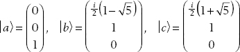
1. The eigenvalues of σx are {1, −1} and the normalized eigenvectors are
To construct a unitary matrix to diagonalize σx, we use the eigenvectors for each column of the matrix, that is,
2. The eigenvalues are (2, i, −i) and the (unnormalized) eigenvectors are

The matrix which diagonalizes X is constructed from these eigenvectors (but normalize them)
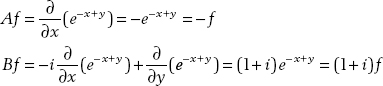
3. (a) Noting that partial derivatives commute, we have

(b) To find the eigenvalues, apply each operator to the given function. We see that the eigenvalue of B is (1 + i)

4. Write down the Taylor series expansions of the exponentials.
5. Will work if F is a real function.
6. (a) Use  and [x, p] = xp − px = i
 to find

(b) Use  then expand f(x) in a Taylor series, using [x, p] = xp − px = i to show that the second term is zero.
7. (a) Noting that partial derivatives commute, we have

(b) To find the eigenvalues, apply each operator to the given function. We see that the eigenvalue of B is (1 + i)
8. (a) The matrix representations of each operator are
(b) These are projection operators, as can be seen by checking the requirements projection operators must meet. For example, consider the square of each operator. Noting that the set is orthonormal, we have

Since P2 = P in both cases, they are projection operators.
(c) First we check the normalization
Since the inner product does not evaluate to 1, the state is not normalized. We divide by the square root of this quantity to get a normalized state, which we denote with a tilde. The matrix representation of the state is
(d) Using the outer product notation, we have
Using matrices

Chapter 8
1. Applying the matrix to each basis vector we obtain
2. The expectation value is found by calculating 

3. The density matrices are formed from
(a) 
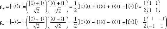
(b) In this case the density operator is
It is a good idea to verify that the trace of each matrix representing these density operators is 1, as it should be.
(c) To see if the state is pure or mixed we square each matrix and compute the trace
The probabilities are found by calculating  , and
, and  . For example

4. (a) To determine if this is a pure state, we square the density operator and compute the trace
Therefore we find that
This means that this density operator represents a mixed state.
(b) First we calculate
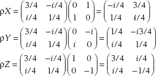
We obtain the components of the Bloch vector by taking the trace of each of these matrices

The magnitude of the Bloch vector is
Since  this is a mixed state.
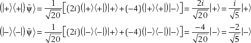
(c) The probability is found by calculating Tr(p1p)

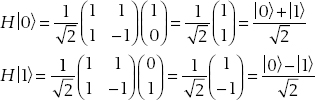
5. (a) 
(b) We compute the inner product and set it equal to 1, and solve for A
(c) The matrix representation is given by

(d) The column vector is

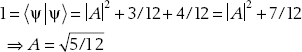
(e) Using the Born rule the probabilities are

Notice that these probabilities sum to one
5/12 + 1/4 + 1/3 = 1
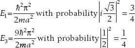
(f) We can find the average value of the energy we can use  where pn is the probability of finding energy En. This gives
(g) The state changes with time according to  and so we have
Chapter 9
1. (a) Using the fact that the basis states are orthonormal, we calculate  giving
Solving we find that 
(b) The energy for the state  of the harmonic oscillator is
  . The possible energies that can be found in the given state and their respective probabilities are

(c) The state at a later time t can be written as
2. Follow the procedure used in Example 9-6. In particular, use [a, a†] = aa† − a†a = 1 to write
3. Starting by writing the Hamiltonian operator in terms of the ladder operators,
However, we know that
We can equate this to  and divide through by ω. This allows us to write
4. Write the Hamiltonian in terms of the number operator and consider the fact that  . Then consider the ground state.
5. We write the number operator explicitly and then use [A, B] = −[B, A] and [A, BC] = [A, B] C + B [A, C]. In the first case this gives
For the other commutator we obtain
6. In the coordinate representation, we have

The expectation value of x in any state is going to be
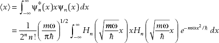
This integral can be rewritten using
Then we recall that the Hermite polynomials satisfy
Note the presence of the Kronecker delta δmn in this formula. This means that if m ≠ n the integral vanishes. In particular, you will find that  = 0 in the ground state (or consider that the integral you will obtain is of an odd function over a symmetric interval—so it must vanish).
For momentum, write the momentum operator in coordinate representation (that is, as a derivative) and consider the relation
together with the integral formula for the Hermite polynomials.
Chapter 10
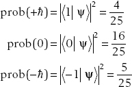
1. First write down the basis states

The possible results of measurement are + , 0, and −
 . The probabilities of obtaining each measurement result are obtained by applying the Born rule, and are given in turn as
  , and
, and  . Proceeding, using the particle state given in the problem the first inner product is

Therefore the probability of obtaining measurement result + is

Next, we find that
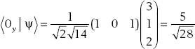
So the probability of obtaining measurement result 0 is
Finally, we have

So the probability of finding measurement result − is

The reader should verify that these probabilities sum to one.
2. (a) It is easier to find N if we write the state in Dirac notation
Using  we find that
  .
.
(b) Incorporating the normalization constant into the state we have
Then using the Born rule the probabilities are
(c) The ladder operators act on the basis states according to

So we find that

3. With J = 2 we can have m = −2, −1, 0, 1, 2.
4. We begin by applying a famous trig identity
Now use Euler’s formula
Using 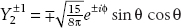 we arrive at the final result
5. C
Chapter 11
1. C
2. D
3. C
4. B
5. C
6. A
Chapter 12
1. C
2. A
3. C
4. A
5. B
Chapter 13
1. B
2. 
3. 14K
4. 3K
5. The electrons would all occupy the ground state with n = 1, l = 0, m = 0
6. 2 electrons
7. 6 electrons
8. (1s)2(2s)2(2p)4
9. (1s)2(2s)2(2p)6
10. 10
Chapter 14
4. B
8. C
9. C
10. B
Chapter 15
1. 0
3. D
4. A
5. B
6. D
7. C
8. D
9. B
10. A
Chapter 17
2. B
3. A
4. C
5. D
Final Exam Solutions
1. D
2. C
3. A
4. C
5. D
6. B
7. B
8. A
9. D
10. B
11. D
12. A
13. D
14. D
15. C
16. E
17. A
18. B
19. D
20. C
21. C
22. B
23. B
24. D
25. A
26. B
27. C
28. B
29. C
30. B
..................Content has been hidden....................
You can't read the all page of ebook, please click here login for view all page.