

chapter 13
Identical Particles
We now consider the study of two-particle systems in detail. We will find that many of the basic or fundamental principles of quantum mechanics carry over to the study of two-particle systems; however, we will see that there are two classes of particles in nature with very different properties. These are known as fermions and bosons. We will get into the differences between these in a moment, but for now let’s go over some of the basics of two-particle systems.
CHAPTER OBJECTIVES
In this chapter you will
• learn about the hamiltonian for systems of two or more identical particles
• learn about the two general types of particles, fermions and bosons
• construct the wavefunction for fermions and bosons
• see how the Pauli exclusion principle constrains the behavior of fermions
Basic Principles of Systems of Identical Particles
Before getting into abstract formalism with bras and kets, we return to basics in terms of wavefunctions and the Schrödinger equation. And at first we won’t worry about identical particles per se. So we’ll think of two-particle systems in terms of wavefunctions. First let’s recall that a wavefunction ψ can depend on position and time. To consider the case of a particle moving in two or three dimensions, we’ll denote position by the vector r and write
Now, if there are two particles, they will each have independent positions. We can denote these by r1 and r2. The time coordinate t will be the same for both particles. Hence the wavefunction will be a function of all three variables, that is,
Everything we know about wavefunctions carries over at this point. The wavefunction must satisfy the Schrödinger equation:
where  is the Hamiltonian operator:
However, we must modify the operator on the left-hand side a bit to take into account that each particle has its own spatial coordinates. First we’ll have to modify the spatial derivatives in the Schrödinger equation, considering the multiple-dimension case. That means that each particle 1 and particle 2 will have its own laplacian operator, and we will assume that each particle has its own mass. We label the masses of each particle m1 and m2. So the following change must be made:
Furthermore, we must account for the potential V acting at the two different spatial positions. This means that
All together we have

Now let’s turn to the Born interpretation, which teaches us that the wavefunction is about probability. Recall that the magnitude squared of the wavefunction gives the probability of finding it within a given spatial location. That is, in a single spatial dimension x, the probability of finding a particle between x and dx is
And the wavefunction must be normalized, which is another way of saying that the probabilities sum to unity:
Carrying this over to the two-particle case in multiple dimensions, we see that the probability of finding particle 1 in the volume d3r1 and particle 2 in the volume d3r2 is given by the the magnitude squared of the wavefunction:
Furthermore, we want the wavefunction to be normalized in the usual way:
Fermions and Bosons
So far we haven’t really learned anything new, but now we’re going to change gears a bit and suppose that the two particles in question are the same type of particle. In other words, they could be two electrons, two neutrons, or two photons, as possible examples.
When you make this leap, there are some peculiar properties of wavefunctions that make the study of identical-particle systems a little more interesting as opposed to rehashing all the same stuff. The changes we’re going to encounter come from the notion of distinguishability.
In classical physics, while particles of the same type have the same properties—mass, charge, and density, say—it is possible, at least in principle, to imagine being able to label individual particles in some way. Not only does each particle have a definite, unique trajectory, but also we can imagine labeling them with some kind of tack to track each particle’s motion independently. Imagine studying the motion of two rubber superballs in a closed room. The two superballs could be the same, made of the same material (having the same density), having the same size, and so on. But we could paint one ball blue and the other yellow and then follow their trajectories.
In the real microscopic world—and hence in the world of quantum mechanics—such tagging or labeling of particles is not possible. One electron cannot be distinguished from another electron in any way. More generally, identical particles (of any type, not just electrons) cannot be distinguished in a quantum system. We also know that we cannot completely determine the trajectory of a given particle because of the uncertainty principle. These two facts have profound consequences for quantum systems.
Mathematically, this means that a wavefunction for two identical particles can’t give us a means to distinguish between them. Put another way, we can’t know which particle is at position r1 and which one is at position r2 until we actually make a measurement. Or if we were studying spin, we couldn’t know which particle was spin-up and which one was spin-down. So we’ll need to build a wavefunction in such a way that accounts for these different possibilities. First let’s start by assuming that the wavefunction is a product of the individual wavefunctions for each particle (look at the time-independent case for now):
Now if we can’t say which particle is at which position, then the following case would also be valid:
Now how do we account for such a situation in quantum mechanics? We take the superposition of the different possibilities. There are two ways we could do this—we could add the two wavefunctions, or we could subtract them. If we let A be an overall normalization constant, this means that the possible wavefunctions we can construct are
The distinction leads to two general classes of particles that exist in physics, and the primary way that they are distinguished is by the type of spin that the particles can have. If we take the plus sign, we say that the particles in question are bosons:
A boson has an integer spin; hence it could be 0, 1, 2, and so on. Examples of bosons in the real world include photons and the as yet hypothetical graviton. Generally speaking, bosons are mediators of physical forces such as electromagnetism.
On the other hand, if we take the minus sign, we end up with fermions:
Fermions have half-integral spin, such as spin-½. When you think of fermions, think of matter. That is, while bosons mediate forces between matter particles, the particles themselves are fermions. Examples of some fermions you’re familiar with include electrons and neutrons (although a neutron is a composite particle made of three quarks, which are themselves fermions).
You will often hear that a quantum state is completely symmetric or completely antisymmetric. A state is completely symmetric if we can swap the wavefunctions of the particles without any overall sign change for the wavefunction of the system. So, bosons are described by completely symmetric states. To see this, note that we are talking about making the following changes:
Hence we write a wavefunction that would describe bosons:
Making the exchange described above, we end up with the same wavefunction:
Now let’s do the same exercise with an antisymmetric wavefunction, that is, a wavefunction for two identical fermions. Remember, we have a minus sign in this case:
Now take
and we get
Hence, in the antisymmetric case we pick up an overall minus sign.
Wavefunctions for fermions are antisymmetric, so swapping particles will introduce an overall minus sign. Wavefunctions for bosons are symmetric, so there will be no change in overall minus sign. For a two-particle system, you can recognize fermions from the minus sign, i.e.,  while a wavefunction for bosons will look like this:
Now let’s discuss this in terms of the bra-ket formalism. First, let’s consider a two-particle system made up of distinguishable particles. If the particles could be in states  and
and  , then we could have a state
This is clearly a different state from the one where particle 1 is in state and particle 2 is in state  :
:
The inner product between the states is
Of course if states and are orthogonal, then  = 0.
= 0.
We can describe the permutation of states by the action of a permutation operator that we will denote as  . Basically, the permutation operator acts on states in the following way:
It must be true that applying the permutation operator twice is the same as the identity operator:
This follows because
Now let’s see how the permutation operator acts on bosons and fermions, that is, on completely symmetric and completely antisymmetric states. First let’s write down a completely symmetric state:
where the plus subscript denotes that this is a symmetric state. In this case, we have
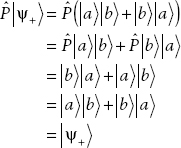
Therefore we can write
We’ve found that completely symmetric states of bosons are eigenstates of the permutation operator with eigenvalue +1. Now let’s consider the action of the permutation operator on completely antisymmetric states of fermions:

where the minus subscript denotes an antisymmetric state. And so we have
So we have found that completely antisymmetric states (fermions) are eigenstates of the permutation operator with eigenvalue −1. Remember how spin relates to bosons and fermions. We can also say that particles with integer spin have eigenvalue +1 for all permutation operators while particles with half-integer spin have eigenvalue −1 for all permutation operators.
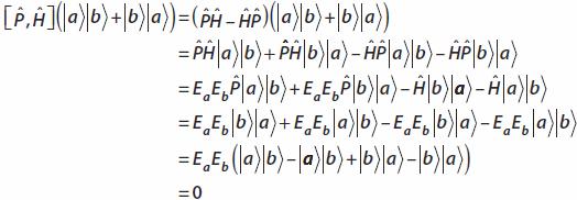
Now the states in question will be eigenstates of some Hamiltonian H. Since they are also simultaneous eigenstates of the permutation operator, it follows that the permutation operator commutes with the Hamiltonian:
Note that the permutation operator also goes by the name exchange operator.
The Pauli Exclusion Principle
The Pauli exclusion principle is important for understanding many physical phenomena such as the way electrons fill the orbitals in an atom. What this principle tells us is that two identical fermions cannot have the same state (i.e., have the same eigenvalues) for a complete set of observables. For instance, two fermions in a given system cannot have the same energy. If you had two fermions trapped in an infinite square well, they could not both be simultaneously in the ground state, or both be simultaneously in the first excited state. You could, however, have one particle in the ground state and one in the first excited state. For bosons, however, you could have both particles simultaneously in the ground state. This has enormous practical physical consequences, e.g., telling us possible energies that fermion or boson systems can have.
This result follows because in an antisymmetric system if both particles were in the same state, the wavefunction for the entire system would vanish, whereas in a symmetric system it will not. This is easy to see. Let’s look at bosons first. We have a state with the following form (ignoring normalization):
Now let’s put both particles in the same state:
We just get
Now look at the antisymmetric case, which describes fermions. Remember in this case we’ve got a minus sign in the wavefunction (again ignoring normalization):
Now let both particles be in the same state, say,
Then
This is a mathematical statement of the fact that fermions cannot be in the same state.
Fermions obey Pauli’s exclusion principle, meaning that two particles cannot have the same quantum numbers, and fermions have half-integral spin. Bosons do not obey the Pauli exclusion principle, and they have integral or zero spin.
Show that
by explicit calculation, using a completely symmetric state. Here the Hamiltonian acts on both states:
Consider two bosons in a two-dimensional infinite square well of width a. Describe the first two states and their energies, ignoring normalization.
First, let’s recall that a particle in an infinite square well has a state of the form (ignoring normalization)
with energy
where n is a positive integer. If there are two particles in the square well, the state will be a product of the individual wavefunctions:
with energy
For bosons, we must construct states as a superposition, with a plus sign:
Since the particles are bosons, it’s possible for both of them to be in the ground state simultaneously. Hence, the lowest energy state for this two-particle system is given by
(recall the state is not normalized). The energy of the state is
The first excited state will be a superposition. The two possibilities are that the first particle is in the (single-particle) ground state, and the other particle is in the (single-particle) first excited state; or the first particle is in the (single-particle) first excited state, and the second particle is in the (single-particle) ground state. In other words,
The energy of the first excited state for the composite system is
Contrast Example 13-2, with the fermionic case, if the particles have no spin. Again, don’t worry about normalization.
Two fermions cannot occupy the same state. If both particles were in the ground state, we would have
So the state with energy
cannot exist for two fermions trapped in an infinite square well. Of course, the Pauli exclusion principle tells us this, since the two electrons cannot have the same energy. Therefore, the ground state for the fermion case will be the one with one particle in the single-particle ground state and the other particle in the single-particle first excited state. The state of the system is
Note again that we have ignored normalization. The energy of the ground state for the fermion case is
The Periodic Table
The Pauli exclusion principle and the fact that particles in nature are either bosons or fermions help us explain the periodic table in chemistry. This is so because the Pauli exclusion principle determines the electron structure of atoms. As we alluded to earlier, it determines how electrons fill available energy levels in the atom. Electrons in atoms can be described by four quantum numbers:
• n: This is the principle quantum number, which tells us which energy level the electron is occupying
• l: Orbital angular momentum
• ml: Magnetic quantum number
• ms: Spin quantum number
The primary designation of a shell in an atom is the primary quantum number n. For a given energy level described by n, there are a number of subshells that are determined by the value that angular momentum can assume:
l = 0, 1, 2, …, n − 1
Each subshell l has subshells according to the values that ml can assume, which are defined according to
ml = −l, −l + 1, …, l −1, l
(For the reasons behind this, please review Chap. 10 on angular momentum.) In each of these subshells, an electron could be spin-up or spin-down. So each subshell specified by the state  can contain two electrons.
So energy levels in atoms are filled with as many electrons as possible, with each electron defined by a unique state or set of quantum numbers. This is how atoms with increasing numbers of protons—and hence numbers of electrons—fill their energy levels and give the structure of the periodic table. We start with hydrogen, with one electron. The lowest energy state is
For historical reasons, it is common in the literature to identify states by letters, such as s, p, and d. These are defined as follows:
• s State: 1 orbital, l = 0, ml = 0.
• p State: 3 orbitals, a p state is l = 1, hence the 3 orbitals come from ml = −1, 0, 1.
• d State: 5 orbitals. A d state is l = 2, hence the 5 orbitals come from the possible values ml = −2, −1, 0, 1, 2.
Now how many electrons can each orbital contain? Each orbital can contain two electrons, one spin-up and one spin-down. That way each electron has a unique state as defined by all four quantum numbers. So
• s State: 1 orbital, can be occupied by 2 electrons
• p State: 3 orbitals, can be occupied by 6 electrons
• d State: 5 orbitals, can be occupied by 10 electrons
The letters are simply another way of identifying the angular momentum l. So states identified by nl are indicated as 1s, 2s, 2p, etc.
What is the maximum number of electrons that can occupy a given orbital?
For a given angular momentum l, there are 2l + 1 possible states. Recall that 2l covers the range of possible values of angular momentum from l − 1, …, 0, …, l + 1 and is the number of values of ml. An electron can be spin-up or spin-down, so each state can have two electrons. So a state can have a maximum of 2(2l + 1) electrons.
For an atom in the ground state, electrons simply fill the orbitals in order of increasing energy. Recalling that for energy level n we can have
l = 0, 1, 2, …, n − 1
possible values for angular momentum. So for the lowest energy level, there is only one value l = 0, and we can put a maximum of two electrons—one spin-up and one spin-down. This corresponds to the 1s state. For hydrogen, there is just one electron, so for hydrogen we have the 1s state. We indicate the total numbers of electrons in a state by a superscript. So for hydrogen we write
1s1
Helium has two electrons. There is still one spot available in the 1s state, so the added electron simply fills in the next available state, giving two electrons in the 1s state:
1s2
Now let’s consider lithium, which has three electrons. The 1s state is completely filled by the first two electrons. The next energy level, n = 2, can have l = 0, 1. We look at each orbital in turn, so first we take l = 0. This is the 2s orbital. So lithium has two electrons in the lowest 1s state and one in the next state up, 2s. We write the configuration as follows:
1s2 2s1
Now let’s consider a more complicated case. Take nitrogen, which has seven electrons. We have room for one more electron in the 2s state, allowing us to account for four of the electrons. To take account of the other three, we have to look at l = 1. Here there are three possible subshells, defined by
ml = −1, 0, 1
This is the 2p state. We can put one electron for each of the ml values, so nitrogen will have two electrons in the 1s state, two electrons in the 2s state, and three electrons in the 2p state. We write this as
1s2 2s2 2p3
The leading numbers denote the value of n in each case.
Using the Pauli exclusion principle, explain how many electrons can fill a p orbital.
A p orbital corresponds to the case
ml = −1, 0, 1
For each value of ml we can have a spin-up electron and a spin-down electron. So there can be two electrons in each subshell, or 3 × 2 = 6 total electrons.
More General Cases
So far we’ve looked at two-particle systems, but the same principles apply to multiparticle systems of any number. Let’s consider three particles. For bosons, a three-particle system would be described by the symmetric state:
The leading square root comes from normalization. For fermions, the state will be antisymmetric:
In general, for N identical bosons, the state will be a superposition of N ! possible arrangements of the states:
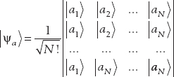
For the antisymmetric or fermion case, the state is given by the Slater determinant:
Summary
In this chapter we learned that
• Identical particles cannot be distinguished in quantum physics.
• There are two general classes of particles. Particles with antisymmetric wavefunctions are called fermions, while particles with symmetric wavefunctions are called bosons.
• Fermions obey the Pauli exclusion principle, but bosons do not.
• Fermions have half-integral spin.
• The spin for bosons can be 0 or an integer.
• The Pauli exclusion principle helps explain why electrons fill atomic orbitals the way they do, and it is an indispensable tool for understanding not just physics but also chemistry.
QUIZ
1. Which of the following particles will have a positive eigenvalue with respect to the permutation operator?
A. Quarks
B. Higgs boson
C. Neutron
D. Electron
2. Describe the action of the permutation operator on the state
3. Three fermions are confined in an infinite one-dimensional square well. Find the energy of the ground state.
4. Three bosons are confined in an infinite one-dimensional square well. Find the energy of the ground state.
5. If electrons were bosons, how would the atomic energy shells be filled?
6. How many electrons can occupy an s state in an atom?
7. How many electrons can occupy a p state in an atom?
8. Describe the orbitals of oxygen, using s, p, d notation and the Pauli exclusion principle.
9. Describe the electron orbitals for neon.
10. Using the Pauli exclusion principle and the four quantum numbers, deduce the maximum number of electrons that can fill a d orbital.
..................Content has been hidden....................
You can't read the all page of ebook, please click here login for view all page.